title: Measurement of the $t\bar{t}t\bar{t}$ Production Cross Section at 13 TeV ...

With the discovery in 2012 of the last predicted elementary particle of the SM, the Higgs boson, particle physics has entered uncharted waters. On one hand, a new heavy particle, or particles, may still be produced and observed in one of the many signatures already being explored at the LHC. Alternatively, that new particle may be too heavy or have some other property that makes direct production and observation infeasible, but its existence influences the behavior of SM processes in ways that may be difficult to measure or are very rare. One such rare process is the production of four top quarks.

Featuring high jet multiplicity and up to four energetic leptons, four top quark production is among the most spectacular SM processes that can occur at the LHC. It has a production cross section of $12.0^{+2.2}{-2.5}$ fb calculated at NLO at 13 TeV center of mass energy[@Frederix2018]. Previous analyses performed by ATLAS[@Aaboud2018;@Aaboud2019] and CMS[@Sirunyan2017;@Sirunyan2018;@1906.02805] have resulted in four top quark production cross section measurements of $28.5^{+12}{-11}$ fb from ATLAS and $13^{+11}_{-9}$ fb from CMS. The goal of this analysis is to improve upon previous results by analyzing a larger data set and utilizing improved analysis methods. This more precise measurement will be used to constrain the top quark Yukawa coupling and masses of heavy mediators in a Two-Higgs Doublet Model.

Production Mechanisms of $t\bar{t}t\bar{t}$

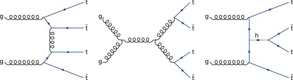
The production of four top quarks can proceed through both strong and electroweak interactions. [@Fig:ft_prod_feyn] shows a few representative Feynman diagrams. As discussed in chapter 2, perturbative calculations of cross sections are performed to a certain order of the relevant coupling constant. For example, processes that only involve the strong interaction can be calculated to $\mathcal{O}(\alpha_s)$, $\mathcal{O}(\alpha_s^2)$ and so on, where the exponent equates to the number of strong vertices in each Feynman diagram included in the calculation. However, one can also consider processes that involve different types of interactions. This leads to mixed order calculations where there are a certain number of QCD vertices, and a certain number of electroweak vertices.

At LHC energies, LO calculations are typically done up to $\mathcal{O}\left(\alpha_s^i \alpha^j\right)$, where $i$ and $j$ are the smallest integers that give a non-vanishing cross section, and $\alpha$ is the electroweak coupling constant. The NLO calculation can involve just adding an additional QCD vertex or external line, leading to $\mathcal{O}\left(\alpha_s^{i+1} \alpha^j\right)$. Doing this improves the accuracy of the total cross section substantially, but the precision of certain parts of the differential cross section will suffer, due to the missing electroweak NLO contribution which contribute preferentially in those areas. These missing contributions make the differential cross section, or rather simulated events based on it, inappropriate for comparison with recorded events. Therefore, significant theoretical work was done to arrive at the "full-NLO" prediction quoted at the beginning of this chapter. The diagrams in [@fig:ft_prod_feyn] shows gluon initial state production, also referred to as gluon fusion. Approximately 90% of the $t\bar{t}t\bar{t}$ cross section is from this process, with the remainder accounted for by quark initial state diagrams, including both the up and down valence quarks and heavier sea quarks. The contribution to the total cross section from vector boson and Higgs boson mediated diagrams is small compared to the QCD contribution. However, as will be discussed in [section @sec:top_yukawa], the contribution from the Higgs boson mediated diagrams can become significant if the top quark Yukawa coupling is larger than its SM value.

{#fig:ft_prod_feyn}

Decay of the $t\bar{t}t\bar{t}$ System

As discussed in chapter 2, top quarks almost always decay to an on-shell W boson and a bottom quark. Therefore, the final state particles of an event with top quarks are determined by the decay mode of the child W boson, since the bottom quark will always form a jet. Approximately 67% of W bosons decay to lighter flavor (i.e. not top) quark pairs, while the rest will decay to $e$, $\mu$, and $\tau$ leptons in approximately equal probability, each accompanied by its matching flavor anti-neutrino. Electrons and muons can be observed directly while tauons will immediately decay to either a lighter charged lepton plus neutrino, or to hadrons.

For a single top quark, then, the potential final states are: \begin{align} t &\rightarrow W^+(\rightarrow e^+ + \nue) + b &(11\%) \ t &\rightarrow W^+(\rightarrow \mu^+ + \nu\mu) + b &(11\%) \ t &\rightarrow W^+(\rightarrow \tau^+(\rightarrow e^+ + \nue + \bar{\nu}\tau) + \nu\tau) + b &(2\%) \ t &\rightarrow W^+(\rightarrow \tau^+(\rightarrow \mu^+ + \nu\mu + \bar{\nu}\tau) + \nu\tau) + b &(2\%) \ t &\rightarrow W^+(\rightarrow \tau^+(\rightarrow \mathrm{quarks} + \bar{\nu}\tau) + \nu\tau) + b &(7\%) \ t &\rightarrow W^+(\rightarrow q + \bar{q}') + b &(67\%) \ \end{align} where the number in parentheses indicates the relative abundance, or branching ratio, of each decay mode.

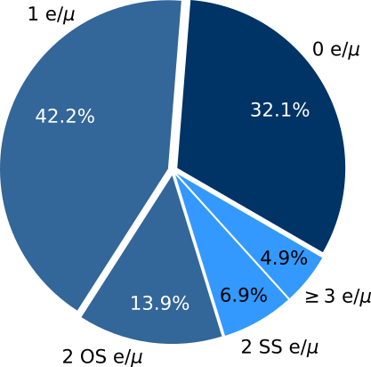
For four top quarks, the final states are conventionally defined in terms of the number and relative charges of final state leptons (including tauon decay products). This is summarized in [@fig:ft_final_states] with the coloring indicating three categories: fully hadronic, single lepton or opposite-sign dilepton[^1], and same-sign dilepton or three or more leptons, where lepton here and henceforth should be taken to mean electron or muon unless otherwise noted.

[^1]: dilepton: a pair of leptons, here meaning a pair consisting of electrons and muons in any combination.

{#fig:ft_final_states}

Analysis Strategy

Four top quark searches for each of these final state categories demand unique analysis strategies due to different event content and vastly different SM backgrounds. In particular, the same-sign dilepton and three or more lepton category benefits from a relatively small set of SM backgrounds at the expense of a rather small overall branching ratio. This is the category that is examined in this analysis[^2].

[^2]: The analysis description in this document omits some details for the sake of clarity. However, the analysis documentation[@CMSFT2019] contains all the technical details.

The strategy of this analysis is to first craft a selection of events that are enriched in $t\bar{t}t\bar{t}$. This is done by making selections based on relatively simple event quantities such as the number and relative sign of leptons, number of jets, number of jets identified as originating from a bottom quark (b-jets), overall hadronic activity, and missing transverse momentum. A multivariate classifier(MVA) is trained on simulated events within this selection to distinguish $t\bar{t}t\bar{t}$ from background events. This MVA produces a discriminant value that tends towards one for $t\bar{t}t\bar{t}$-like events, and to zero for background-like events. The range of values that this discriminant can take is divided into several categories, or bins. Each event is placed within one of these bins based on its discriminant value. Finally, a maximum likelihood fit is performed on the distribution of events in the discriminant bins to extract the deviation of the measured distribution from the background-only hypotheses. A statistically significant (and positive) deviation can then be interpreted as evidence of $t\bar{t}t\bar{t}$ production, and can be further processed to find a cross section measurement.

Data Sets and Simulation

This measurement uses data collected from 2016-2018 with the CMS detector corresponding to a total integrated luminosity of 137.2 fb$^{-1}$. Events that pass the HLT are divided into roughly disjoint data sets. Of the many of these produced by CMS, this analysis uses:

DoubleEG: Events that contain at least two energetic electrons
DoubleMuon: Similar to DoubleEG, except requiring muons instead of electrons
MuonEG: Crossed channel including events with one muon and one electron

Because the data sets are not completely disjoint, care has been taken to avoid double counting events that may occur in multiple data sets.

Monte Carlo simulation is used extensively to model background and signal processes relevant to this analysis. See chapter 4 for more details on the process of producing simulated events. Samples of simulated Standard Model processes are produced centrally by a dedicated group within the CMS collaboration. The primary samples used in this analysis are listed in [table @tbl:samples]. Because detector conditions were changed year-to-year, this analysis uses three sets of samples, one for each year.

Process	Cross section (pb)
$t\bar{t}t\bar{t}$	0.01197
Drell-Yan: $q\bar{q}\rightarrow l^+l^-$, $10<m_{ll}<50$ GeV	18610
Drell-Yan: $q\bar{q}\rightarrow l^+l^-$, $m_{ll}>50$ GeV	6020.85
$W$ + jets	61334.9
$t\bar{t}$	831.762
$t\bar{t}W$, $W\rightarrow \ell \nu_\ell$	0.2043
$t\bar{t}Z$, $Z\rightarrow \ell^+ \ell^-$ or $Z\rightarrow \nu\ell \bar{\nu}\ell$	0.2529
$t\bar{t}H$, $H\nrightarrow b\bar{t}$	0.2710
$tZq$, $Z\rightarrow \ell^+\ell^-$	0.0758
$tbq\gamma$	2.967
$t\bar{t}\gamma$	2.171
$W\gamma$, $W \rightarrow \ell \nu_\ell$	405.271
$Z\gamma$, $Z \rightarrow \ell^+ \ell^-$	123.9
$WZ$, $Z\rightarrow \ell^+ \ell^-$, $W\rightarrow \ell \nu_\ell$	4.4297
$ZZ$, $Z\rightarrow \ell^+\ell^-$ $\times 2$	1.256
$ZZZ$	0.01398
$WZZ$	0.05565
$WWZ$	0.1651
$WZ\gamma$	0.04123
$WW\gamma$	0.2147
$WWW$	0.2086
$WW$, $W\rightarrow \ell \nu_\ell$ $\times 2$	0.16975
$tW\ell^+\ell^-$	0.01123
$W^+W^+$	0.03711
$ggH$, $H\rightarrow ZZ$ $Z \rightarrow \ell^+ \ell^-$ $\times 2$	0.01181
$WH$/$ZH$, $H\nrightarrow b\bar{t}$	0.9561
$t\bar{t}HH$	0.000757
$t\bar{t}ZH$	0.001535
$t\bar{t}ZZ$	0.001982
$t\bar{t}WZ$	0.003884
$t\bar{t}tW$	0.000788
$t\bar{t}tq$	0.000474
$t\bar{t}WH$	0.001582
$t\bar{t}WW$	0.01150

: Primary simulated samples used in this analyses. Each process is inclusive of all final states unless specified otherwise. {#tbl:samples}

Because the number of jets, $N_{jet}$, is expected to be an important variable for separating $t\bar{t}t\bar{t}$ from background events, it is important to ensure that the spectrum of the number of jets originating from initial state and final state radiation (ISR/FSR) is accurately modeled. An ISR/FSR jet originates from a gluon that has been radiated from either one of the initial state partons or one of the final state colored particles. This is particularly true for the major background processes of $t\bar{t}W$ and $t\bar{t}Z$. The key observation to performing this correction is that a mismodeling of the distribution of the number of ISR/FSR jets by the event generator will be very similar between $t\bar{t}W$/$t\bar{t}Z$, and $t\bar{t}$. So by measuring the disparity between data and MC in a selection enriched in $t\bar{t}$, correction weights can be obtained and applied to simulated $t\bar{t}+X$ events.

This correction is obtained as follows. The number of ISR/FSR jets in data is obtained by selecting $t\bar{t}$ events where both child W bosons decayed to leptons and exactly two identified b-jets. Any other jets are assumed to be from ISR/FSR. The weights are then computed as the bin-by-bin ratio of the number of recorded events with a certain number of ISR/FSR jets to the number of simulated events with that number of truth-matched ISR/FSR jets. The results of this measurement for 2016 data and MC are shown in [@fig:isrfsr_correction]. The correction is applied by reweighting simulated $t\bar{t}Z$ and $t\bar{t}W$ events with these weights based on the number of truth-matched ISR/FSR jets.

{#fig:isrfsr_correction}

The number of b-tagged jets is also expected to be an important variable for selecting $t\bar{t}t\bar{t}$ events. Therefore, the flavor composition of additional jets in simulation should also be matched to data. Specifically, there has been an observed difference between data and simulation in the measurement of the $t\bar{t}b\bar{b}/t\bar{t}jj$ cross-section ratio[@CMSttbb]. To account for this, simulation is corrected to data by applying a scale factor of 1.7 to simulated events with bottom quark pairs originating from ISR/FSR gluons. These events are also given a 40% systematic uncertainty on their weights to be consistent with the uncertainties on the ratio measurement.

Object Definitions

This section describes the basic event constituents, or objects, that are considered in this analysis. The choice of the type and quality of these objects is motivated by the final state content of $t\bar{t}t\bar{t}$ events. The objects are electrons, muons, jets, b-jets, and missing transverse momentum. Each of the objects has dedicated groups within the CMS collaboration that are responsible for developing accurate reconstruction and identification schemes for them. The Physics Object Groups (POGs) make identification criteria, or IDs, available for general use in the collaboration. Many analyses, including this one, incorporate these POG IDs into their own particular object definition and selection. This analysis applies additional criteria to define analysis objects. In the case of leptons, two categories are defined: tight and loose, where the former must satisfy more stringent selection criteria than the latter.

Electrons

Electrons are seen in two parts of the CMS detector: the tracker, and the electromagnetic calorimeter. After an electron candidate has been formed by matching an energy deposit in the ECAL with an appropriate track, it is evaluated in one of a variety of schemes to determine the probability that it is from a genuine electron vs a photon, a charged hadron, or simply just an accidental reconstruction from unrelated hits. For this analysis, only electrons with $|\eta|<2.5$, i.e. within both the tracker and ECAL acceptance, are considered.

The particular scheme to determine the quality of an electron candidate employed for this analysis is the MVA ID[@elMvaIdMoriond17;@elMvaIdSpring16;@elMVAFall17] developed by the EGamma POG. The MVA uses shower-shape variables, track-ECAL matching variables, and track quality variables to produce a discriminant. Electron candidates are then required to have a discriminant value above a selection cutoff. Multiple cutoffs are provided with the MVA that define tight and loose working points(WPs).

Charge mismeasurement of leptons can result in an opposite-sign dilepton event appearing as a same-sign dilepton event. Because there are potentially large backgrounds with opposite-sign dileptons, steps are taken to remove events with likely charge mismeasurement. In CMS, there are three techniques for measuring electron charge [@AN-14-164]. These are:

The curvature of the GSF track
the curvature of the general track, obtained by matching the GSF track with general tracks as reconstructed for pions and muons, asking for at least one hit shared in the innermost part (pixels)
The SC charge, obtained by computing the sign of the $\phi$ difference between the vector joining the beam spot to the SC position and the one joining the beam spot to the first hit of the electron track.

A requirement for the highest quality, or "tight", category of electrons used in the analysis is that all three of these methods are required to agree.

The leptons that are desired for defining the event selection are the leptons from the decay of the various top quark's child W bosons. Other leptons, such as those originating in heavy quark decays as part of jets, or from photon pair production are referred to as non-prompt leptons. Photons will sometimes pass through one or more layers of the tracker before undergoing $e^+e^-$ pair-production, resulting in "missing" inner layer hits for the tracks of the child electrons. Tight electrons are therefore required to have exactly zero missing inner hits. Consistency with having originated from the correct p-p interaction is also considered by applying cuts on the impact parameter, or the vector offset between the primary vertex and the track's point of closest approach to it. In particular, there are cuts on $d_0$, the transverse component of the offset, $dz$, the longitudinal component, and $SIP\mathrm{3D}$, the length of the offset divided by the uncertainty of the vertex's position.

Muons

Muons are reconstructed in CMS by matching tracks produced from hits in the muon system to tracks in the tracker. The individual quality of the tracker and muon system tracks as well as the consistency between them are used to define IDs. The Muon POG defines two IDs that are used in this analysis: loose[@MuId], and medium[@muonMediumId]. Only muons within the muon system acceptance $|\eta|<2.4$ are considered, and the same impact parameter requirements are applied as for electrons. For muons, the probability of charge mismeasurement is reduced by applying a quality requirement on the track reconstruction in the form of a selection on the relative uncertainty of the track's transverse momentum: $\delta p_T(\mu) / p_T(\mu) < 0.2$.

Lepton Isolation

Lepton isolation is a measure of how well separated in $\Delta R$ a lepton is from other particles. It is a useful quantity for distinguishing leptons that originate from heavy resonance decays, such as those from $W$ and $Z$ bosons, from leptons that originate as part of a jet. Events from $t\bar{t}t\bar{t}$ and its main backgrounds ($t\bar{t}Z$, $t\bar{t}W$, $t\bar{t}H$) have an especially high number of jets relative to other processes that are typically studied at the LHC. This prompted the development of a specialized isolation requirement, known as multi-isolation[@AN-15-031]. It is composed of three variables.

The first component is mini-isolation[@1007.2221], $I\mathrm{mini}$. To understand the utility of $I\mathrm{mini}$, let us first consider the decay of a top quark where the child W boson decays to a lepton. Depending on the momentum of the top quark, the b-jet and the lepton will be more or less separated, with the separation becoming small at high momentum. Because of this, a constant $\Delta R$ isolation requirement on the lepton will be inefficient for highly energetic particles. Mini-isolation addresses this by utilizing variable cone size. The size of this cone is defined by

$$ \Delta R_\mathrm{cone} = \frac{10}{\mathrm{min}\left(\mathrm{max}\left(pT(\ell), 50\right), 200 \right)} $$ With this, $I\mathrm{mini}$ is $$ I_\mathrm{mini}\left(\ell\right) = \frac{p_T^{h\pm} + \mathrm{max}\left(0, p_T^{h0} + pT^{\gamma} - \rho \mathcal{A}\left(\frac{\Delta R\mathrm{cone}}{0.3}\right)^2\right)}{p_T\left(\ell\right)} $$ where $p_T^{h\pm}$, $p_T^{h0}$, $pT^{\gamma}$ are the scalar sums of the transverse momenta of the charged hadrons, neutral hadrons, and photons, within the cone. Neutral particles from pileup interactions are difficult to separate entirely from neutral particles from the primary interaction. This leads to some residual energy deposition in the calorimeters. The final term in the numerator accounts for this. The $\rho$ is the pileup energy density and $\mathcal{A}$ is the effective area. These are computed using a cone size of $\Delta R\mathrm{cone}=0.3$ and are scaled by the formula appropriately to varying cone size.

The second variable used in the multi-isolation is ratio of the lepton $p_T$ to the $p_T$ of a jet matched to the lepton. $$ p_T^\mathrm{ratio} = \frac{p_T\left(\ell\right)}{p_T\left(\mathrm{jet}\right)} $$ The matched jet is almost always the jet that contains the lepton, but if no such jet exists, the jet closest in $\Delta R$ to the lepton is chosen. The use of $p_T^\mathrm{ratio}$ is a simple approach to identifying leptons in very boosted topologies while not requiring any jet reclustering.

The third and final variable is the relative transverse momentum, $p_T^\mathrm{rel}$. This is the magnitude of the matched lepton's momentum transverse to the matched jet's momentum and then normalized by the jet's momentum: $$ p_T^\mathrm{rel} = \sqrt{|\vec{\ell_T}|^2 - \frac{\left(\vec{\ell_T} \cdot \vec{j_T}\right)^2}{|\vec{j_T}|^2}} $$ where $\vec{\ell_T}$ and $\vec{j_T}$ are the 2-component transverse momentum vectors for the lepton and jet, respectively. This helps recover leptons that are accidentally overlapping with unrelated jets.

The multi-isolation requirement is fulfilled when the following expression involving these three variables is true. $$ I_\mathrm{mini} < I_1 \land \left( p_T^\mathrm{ratio} > I_2 \lor p_T^\mathrm{rel} > I_3 \right) $$ The logic behind this combination is that by relaxing the mini-iso the efficiency of the prompt lepton selection can be improved. The increase in fakes that comes from the relaxation is compensated for by the requirement that the lepton carry the major part of the energy of the corresponding jet, or if not, the lepton may be considered as accidentally overlapping with a jet. The three selection requirements, $I_1$, $I_2$, and $I_3$, are tuned individually for electrons and muons ([table @tbl:multi_iso2016], [table @tbl:multi_iso20172018]), since the probability of misidentifying a jet as a lepton is higher for electrons than muons[@iso_tuning]. After tuning, the selection efficiency for prompt leptons is 84-94% for electrons and 92-94% for muons, and the non-prompt efficiency is 8.1% for electrons and 2.1% for muons.

	loose $\ell$	tight($e$)	tight ($\mu$)
$I_1$	0.4	0.16	0.12
$I_2$	0.0	0.76	0.80
$I_3$	0.0	7.2	7.2

: Isolation requirements used for 2016 {#tbl:multi_iso2016}

	loose $\ell$	tight($e$)	tight ($\mu$)
$I_1$	0.4	0.11	0.07
$I_2$	0.0	0.74	0.78
$I_3$	0.0	6.8	8.0

: Isolation requirements used for 2017 and 2018 {#tbl:multi_iso20172018}

The multi-isolation is used with other quality criteria to define two categories of each flavor of lepton, tight, and loose. The selections for each of these categories is detailed in [table @tbl:lep_selection].

	$\mu$-loose	$\mu$-tight	$e$-loose	$e$-tight
Identification	loose ID	medium ID	loose WP	tight WP
Isolation	loose WP	$\mu$ tight WP	loose WP	$e$ tight WP
$d_0$ (cm)	0.05	0.05	0.05	0.05
$d_z$ (cm)	0.1	0.1	0.1	0.1
$SIP_\mathrm{3D}$ (cm)	-	$<4$	-	$<4$
missing inner hits	-	-	$\le 1$	$=0$

: Summary of lepton selection {#tbl:lep_selection}

Jets

As discussed in chapter 4, jets are reconstructed from particle flow candidates that were clustered with the anti-kt algorithm with a cone size of $\Delta R < 0.4$. To be considered for inclusion in analysis quantities like $N_\mathrm{jets}$, jets must possess a transverse momentum $p_T > 40$ GeV and be within the tracker acceptance $|\eta| < 2.4$. To further suppress noise and mis-measured jets, additional criteria are enforced. For the 2016 data, jets are required to have

neutral hadronic energy fraction < 0.99
neutral electromagnetic energy fraction < 0.99
charged hadron fraction > 0
charged particle multiplicity > 0
charged EM fraction < 0.99

For 2017 and 2018, an adjusted set of requirements were applied. These are

neutral hadronic energy fraction < 0.9
neutral electromagnetic energy fraction < 0.9
charged hadron fraction > 0
charged particle multiplicity > 0

From all jets that pass the stated criteria, a critical variable is calculated that will be used extensively in the analysis, $HT \equiv \sum\mathrm{jets} p_T$.

B-Jets

Hadrons containing bottom quarks are unique in that they typically have a lifetime long enough to travel some macroscopic distance before decaying, but still much shorter than most light-flavor hadrons. This leads to bottom quarks producing jets not originating at the primary vertex but at a displaced vertex. The displaced vertex will typically be a few millimeters displaced from the primary vertex. One of the critical roles of the pixel detector is to enable such precise track reconstruction that the identification of these displaced vertices can be done reliably. This identification of b-jets is done by feeding details of the displaced vertex, and reconstructed jet quantities into a machine learning algorithm that distills all the information to a single discriminant. Different working points are established along the discriminant's domain to provide reference performance metrics. Generally, a loose, medium, and tight WP are defined which correspond to 10%, 1%, and .1% probabilities, respectively, to mis-tag jets from light quarks as bottom quark jets.

In this analysis, jets that pass all the criteria of the previous section, with the exception that the $p_T$ threshold has been lowered to 25 GeV, can be promoted to b-jets. The deepCSV discriminator is used in this analysis at the medium working point[@BTagging].

The jet multiplicity, $N_\mathrm{jets}$, and $H_T$ both include b-jets along with standard jets, provided that they have $p_T>40GeV$.

Missing Transverse Energy

As discussed in chapter 4, neutrinos escape CMS undetected and create an imbalance in the visible transverse momentum of the event. Four top quark events considered in this analysis will have at least two neutrinos which makes this imbalance a useful quantity to use in the event selection. The missing transverse energy is found by calculating the magnitude of the vector sum of the transverse component of the momenta of all PF particles. Corrections to this are made in accordance with the recommendations of the CMS MET working group[@JME-13-003].

Event Selection

Before defining the baseline selection of events, it is good to review what the $t\bar{t}t\bar{t}$ signature is in the same-sign lepton channel.

Two same-sign leptons, including any combination of electrons and muons.
Missing transverse momentum due to the two neutrinos associated with the aforementioned leptons through their parent W bosons
Four b-jets, one from each top quark
Four jets from two hadronic W decays

This analysis is also inclusive of the three and four lepton case. These are similar to the above except there are incrementally more leptons and neutrinos and fewer jets, although the number of b-jets remains constant. With that in mind, the baseline event selection is the following:

a pair of tight same-sign leptons
$N_\mathrm{jets} \ge 2$
$N_\mathrm{b jets} \ge 2$
$E!!!!/_T > 50$ GeV
$H_T > 300$ GeV
$p_{T,\ell1} \ge 25 \mathrm{GeV}, p{T,\ell_2} \ge 20 \mathrm{GeV}$

In the listing, "$\ell_1$" and "$\ell_2$" refer to the tight leptons with the highest and second highest $p_T$, respectively. Additional tight leptons must also have $pT \ge 20$ GeV to count towards $N\mathrm{lep}$.

Events that contain a third lepton passing the loose ID that makes a Z boson candidate with one of the two same-sign leptons are rejected. A Z-boson candidate is formed by an opposite-sign, same-flavor pair of leptons whose invariant mass lies within 15 GeV of the Z boson mass. Low mass resonances are also rejected by applying similar criteria except for the invariant mass being smaller than 12 GeV. However, if the third lepton passes the tight requirements and also creates a Z-boson candidate and has a transverse momentum larger than 5 GeV for muons or 7 GeV for electrons, then the event passes the "inverted Z-veto" and is instead placed into a dedicated $t\bar{t} Z$ control region called CRZ.

If additional tight leptons do not form a Z candidate and have transverse momentum of at least 20 GeV, then they contribute to the lepton count for the event, $N_\mathrm{lep}$.

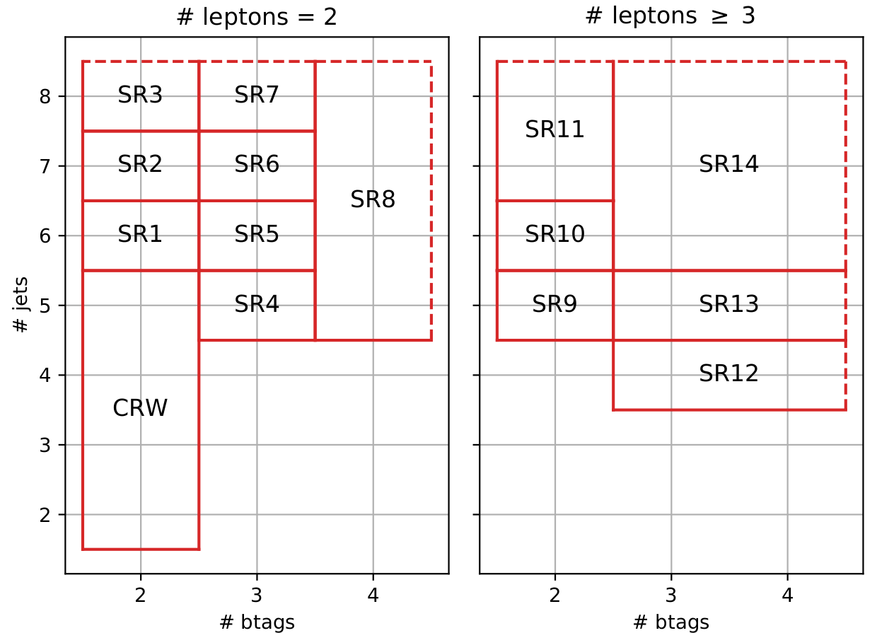
Events that pass the baseline selection and do not get discarded or placed into CRZ are divided into several signal regions. There are two approaches used in this analysis for defining these signal regions.

The first approach, called cut-based, is to categorize the events based on the number of leptons, jets, and b-jets. These regions are described in [@fig:cut_based_sr]. In the cut-based analysis, an additional control region was employed to help constrain the contribution of $t\bar{t}W$ called CRW.

{#fig:cut_based_sr}

The other approach for defining the signal regions is to use an MVA. In this analysis, a boosted decision tree (BDT) was used. This BDT used an expanded set of event information, relative to the cut-based classification, to construct a discriminator that would separate signal, i.e. $t\bar{t}t\bar{t}$, events from all background events. This continuous discriminator value is then discretized into several bins which will each contain events with a discriminator value that lies within the bounds of that bin.

Before the BDT can be used, it must be trained. Due to BDT training being susceptible to overtraining unless a large number of training events are available, a relaxed baseline selection was created to provide additional events for the BDT to train with. The relaxed selection is:

$p_{T,\ell_1} > 15$ GeV
$p_{T, \ell_2} > 15$ GeV
$H_T > 250$ GeV
$E!!!!/_T > 30$ GeV
$N_\mathrm{jets} \ge 2$
$N_\mathrm{b jets} \ge 1$

Signal events were taken from $t\bar{t}t\bar{t}$ simulated samples and background events were taken to be a mixture of simulated SM background processes scaled to their cross sections as listed in [table @tbl:samples]. Over 40 event-level variables were considered for the BDT inputs. These included the multiplicities of leptons, jets, and b-jets passing the tight or loose selection criteria, $H_T$, $E!!!!_T$, transverse momenta of individual leptons and jets, invariant masses and angular separations of pairings of leading and sub-leading leptons and jets, and the number of W boson candidates defined by jet pairs with invariant mass within 30 GeV of the W boson mass.

Of these, the 19 that were determined to have the most discriminating power by the training routine of TMVA[@Antcheva2009] were chosen for further optimization. Additional variables provided no significant increase in discriminating power. This discriminating power is quantified by examining the Receiver Operating Characteristic (ROC) curve. The ROC curve is formed by calculating the signal efficiency and background rejection for different cuts on the discriminator value. Different working points can be defined along this curve, but the discriminator's overall performance can be quantified by calculating the area under the ROC curve (AUC). Of the variables listed above, 19 were chosen to continue optimization.

(a) $N_\mathrm{b jets}$
(b) $N_\mathrm{jets}$
(c) $N_b^\mathrm{loose}$
(d) $E!!!!/_T$
(e) $N_b^\mathrm{tight}$
(f) $p_{T, \ell_2}$
(g) $m_{\ell_1 \ell_2}$
(h) $p_{T, j_1}$
(i) $p_{T, j_7}$
(j) $\Delta\phi_{l_1 l_2}$
(k) $p_{T, j_6}$
(l) $\mathrm{max}\left(m(j)/p_T(j)\right)$
(m) $N_\mathrm{leps}$
(n) $p_{T, \ell_1}$
(o) $\Delta \eta_{\ell_1 \ell_2}$
(p) $p_{T, j_8}$
(q) $H_T^b$
(r) $p_{T, \ell_3}$, if present
(s) $q_{\ell_1}$

Numeric subscripts indicate ranking in the $pT$ ordering of the object. For example, $p{T, j_7}$ is the transverse momentum of the jet with the seventh highest $p_T$. The distributions of these input variables for signal and background processes are shown in [@fig:bdt_kinem].

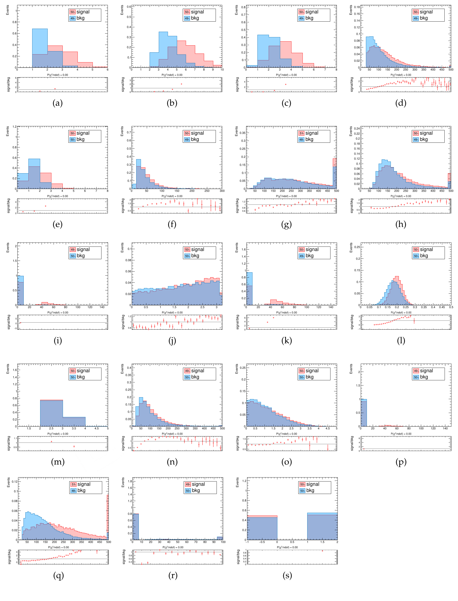{#fig:bdt_kinem}

In addition to the input variables, a BDT is described by several parameters internal to the algorithm. These parameters are referred to as hyperparameters. These change across different MVA algorithms and even between different implementations of the same algorithm. In the case of BDTs in TMVA, the following hyperparameters were chosen and are listed with their optimized values.

NTrees=500
nEventsMin=150
MaxDepth=5
BoostType=AdaBoost
AdaBoostBeta=0.25
SeparationType=GiniIndex
nCuts=20
PruneMethod=NoPruning

An alternative library called xgboost[@Chen:2016:XST:2939672.2939785] was tested for comparison. Optimization of its BDT implementation resulted in the following hyperparameters. Note how this set of hyperparameters is different from those in the TMVA algorithm.

n_estimators=500
eta=0.07
max_depth=5
subsample=0.6
alpha=8.0
gamma=2.0
lambda=1.0
min_child_weight=1.0
colsample_bytree=1.0

[@Fig:bdt_performance] shows a comparison between these two optimized BDTs, and [@fig:xgboost_disc_shape] demonstrates the signal separation achieved by the BDT. The xgboost implementation demonstrates clearly superior performance and was therefore selected for use in this analysis.

{#fig:bdt_performance}

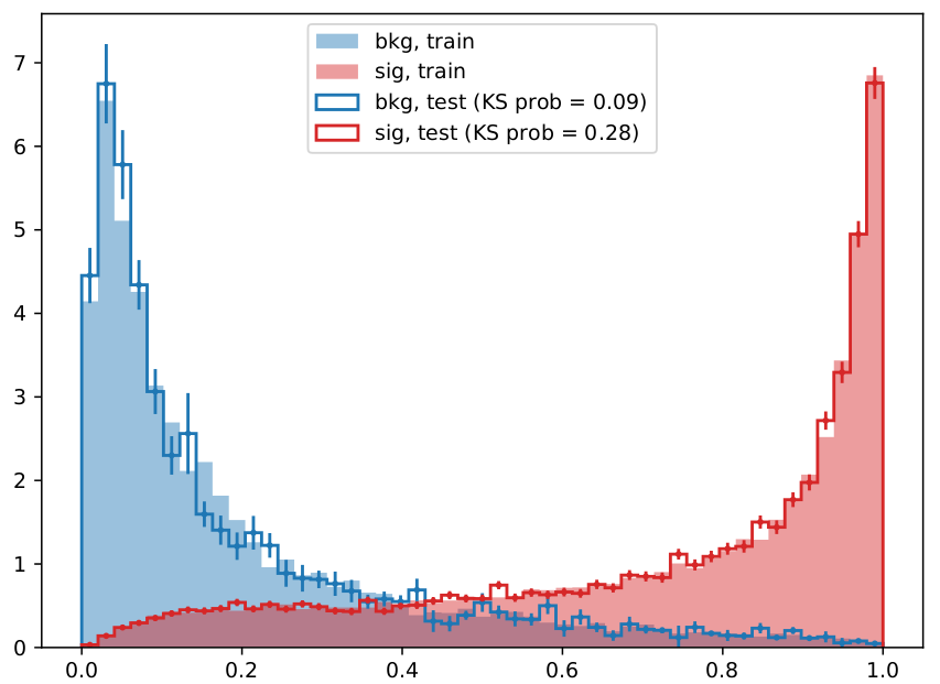{#fig:xgboost_disc_shape}

The analysis that incorporates the BDT discriminant into the signal region definitions is here referred to as the BDT-based analysis. The BDT-based signal regions contain all of the same events as the cut-based signal regions. However, they are distributed into 17 bins based upon the event's discriminant value. The edges of these bins are: \begin{align} [0.0000&, 0.0362, 0.0659, 0.1055, 0.1573, 0.2190, 0.2905, 0.3704, 0.4741, \ 0.6054&, 0.7260, 0.8357, 0.9076, 0.9506, 0.9749, .9884, 0.9956, 1.0000] \ \end{align} In addition, there is 1 bin for events in CRZ, giving 18 bins in total. In contrast with the cut-based signal regions, there is no CRW control region in the BDT analysis. In this case, $t\bar{t}W$ is expected to be constrained in the overall fit, as will be discussed in [section @sec:results].

Background Estimation

An essential ingredient to making an accurate measurement of any cross section is good estimation of background processes. The backgrounds for this analysis can be divided into two main categories: backgrounds with prompt same-sign lepton pairs, and backgrounds with fake same-sign lepton pairs. Of the backgrounds with genuine same-sign prompt leptons, $t\bar{t}W$ and $t\bar{t}Z$ are estimated from simulation and scaled to data with dedicated control regions. For the BDT-based analysis, only $t\bar{t}Z$ has a dedicated control region. Other processes that produce genuine prompt same-same leptons are taken directly from simulation. Data-driven methods are used to construct the contribution of processes producing fake same-sign lepton pairs in the signal and control regions.

Genuine Same-sign Backgrounds

Of the backgrounds that contain authentic same-sign lepton pairs, the most prominent are events from $t\bar{t}W$, $t\bar{t}Z$, and $t\bar{t}H$. Events from these processes are obtained from simulation and scaled to their theoretical cross sections. For $t\bar{t}W$ and $t\bar{t}Z$ a 40% uncertainty on their cross sections is applied, while for $t\bar{t}H$ a smaller 25% normalization uncertainty is taken due to more constraining measurements on the $t\bar{t}H$ cross section[@1712.06104].

In addition to the normalization uncertainties, the shape of the distributions of analysis qualities such as $H_T$, $E!!!!_T$, and jet multiplicity are studied under different choices of simulation parameters. Considered first was the influence of varying the PDFs used in the event generation within their uncertainty bands. The changes in the resulting observable distributions were consistently smaller than the statistical uncertainty from the limited number of MC events. Based on this, no additional uncertainty is assigned for PDF variations. Furthermore, the difference between samples produced using LO and NLO calculations were considered as well as the variation in renormalization and factorization scales. The distributions of events generated at LO and NLO are consistent within their renormalization and refactorization uncertainties, indicating the these uncertainties are sufficient to account for missing contributions from higher-order Feynman diagrams. [@Fig:lo_nlo_shape_compare] shows a comparison between LO and NLO for $t\bar{t}Z$.

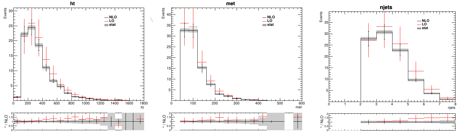{#fig:lo_nlo_shape_compare}

Other background processes with smaller contributions include pairs ($WZ$, $ZZ$) and triplets ($WWW$, $WWZ$, $WZZ$, $ZZZ$) of vector bosons, vector boson(s) produced in association with a Higgs boson ($HZZ$, $VH$), same-sign W pairs from both single and double parton scattering, and other rare top quark processes ($tZq$, $t\bar{t}tW$, $t\bar{t}tq$). The contributions from these processes are grouped together into the "Rare" category. Processes that can produce leptons from an unrecognized photon conversion in addition to other prompt leptons are grouped into a category called "$X+\gamma$". These include $W\gamma$, $Z\gamma$, $t\bar{t}\gamma$, and $t\gamma$. Both the "Rare" and "$X+\gamma$" categories are assigned a large (50%) uncertainty on their normalization due to theoretical uncertainties on their respective cross sections. [@Fig:rares] shows the expected contributions of the processes in the Rare category to the signal regions.

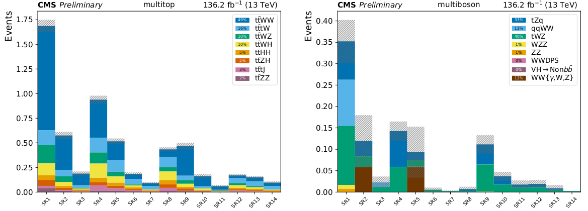{#fig:rares width=99%}

Fake Same-sign Backgrounds

A same-sign lepton pair can be faked in two ways. The first way is for the charge of a lepton to be mis-measured which flips an opposite-sign lepton pair to a same-sign lepton pair. This rate is quite small, but the large number of SM background events that produce opposite-sign lepton pairs makes it important to consider. The second is the production of "non-prompt" leptons. These non-prompt leptons are called such because they are not produced promptly in the initial parton-parton interaction (at the Feynman diagram level), but rather from the decays of longer-lived particles such as charm and bottom flavored hadrons or from lepton pair-production from energetic photons. The definition of non-prompt leptons also includes charged hadrons misidentified as leptons. Leptons that are produced in the initial interaction are called prompt leptons.

The charge misidentification background is estimated by first selecting events in recorded data that pass all signal region selection requirements except for the requirement to have two leading leptons of the same charge. Dimuon events are not considered because the charge misidentification rate for muons is negligible. Selected opposite-sign events are weighted by the probability for each of the electrons with its specific $p_T$ and $\eta$ to have its charge misidentified.

{#fig:charge_flip width=90%}

This probability, shown in [@fig:charge_flip], is measured in simulated events of $t\bar{t}$ production and the Drell-Yan process. It is then validated by selecting recorded events with tight opposite-sign electron pairs with invariant mass near the Z boson mass and $E!!!!_T < 50$ GeV. These events are weighted by the charge flip probability to make a prediction of the number of same-sign events. This prediction is compared to recorded events satisfying the same selection except instead requiring a same-sign electron pair. Further, the same-sign selection is applied to the simulated samples used to measure the flip rate. This is shown in [@fig:charge_flip_validation]. The ratio of the number of events in the same-sign region in simulation and data is used as a scale factor to adjust the flip rates. The scale factor is measured to be 1.01, 1.44, and 1.41 for 2016, 2017, and 2018, respectively.

{#fig:charge_flip_validation width=99%}

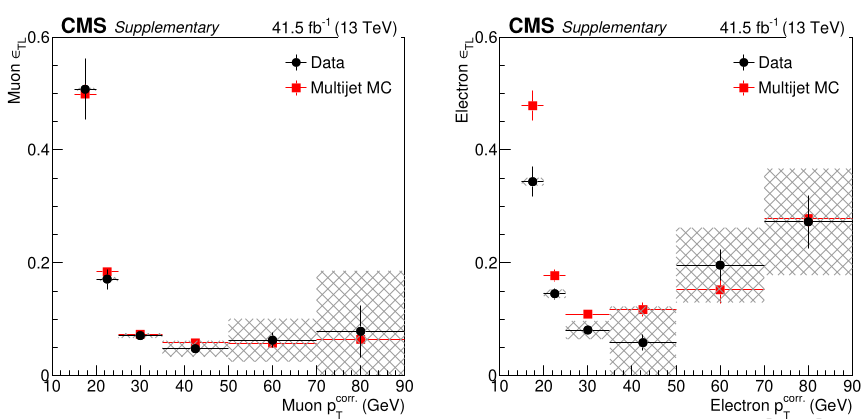
The non-prompt background estimation is similar to the charge misidentification background estimation except that the "fake rate", i.e. an estimate of the probability of a non-prompt lepton to pass the tight ID requirements, is measured not in simulation, but in recorded data.

This method utilizes leptons that pass the loose identification criteria listed in [table @tbl:lep_selection]. The fake rate is then defined as the probability that a lepton that passes the loose set of requirements also passes the tight set of requirements. The fake rate is measured as a function of lepton flavor, $p_T$, and $\eta$. In order to reduce the fake rate's dependence on the $p_T$ of the lepton's mother parton, the $p_T$ used in the fake rate calculation is adjusted[@AN-14-261] as $$ p_T^{\mathrm{cc}} = \begin{cases}

p_T \cdot \left(1+\mathrm{max}\left(0, I_\mathrm{mini} - I_1 \right)\right) ,& p_T^\mathrm{rel} > I_3 \\
\mathrm{max}\left(p_T, p_T(\mathrm{jet}) \cdot I_2\right) ,& \mathrm{otherwise}

\end{cases} $$ where $p_T^{\mathrm{cc}}$ is called the "cone-corrected" $p_T$. This can be understood by considering how a lepton's isolation will change with the mother parton's momentum. As the mother parton's momentum increases, the resulting jet becomes more collimated, decreasing the isolation of the lepton. Adjusting the $p_T$ of the lepton to the cone-corrected $p_T$ provides an estimate of the $p_T$ of the mother parton.

The fake rate is measured with a sample of events enriched in non-prompt leptons. The sample consists of events that have a single lepton that passes the loose requirements, at least one jet with $\Delta R(\mathrm{jet}, \ell) > 1$, $E!!!!/_T < 20$ GeV, and $M_T < 20$ GeV. The transverse mass, $MT=\sqrt{2p{T, \ell} E!!!!/T \left(1 - \cos\left( \phi\ell - \phi_{p!!!/_T} \right) \right)}$, is calculated using the transverse momentum of the lepton and the missing transverse momentum of the event. The requirements on $E!!!!/_T$ and $M_T$ are intended to suppress the contribution of prompt leptons from Z and W boson decays. Despite this, some events with prompt leptons make it into the selection. This "prompt contamination" of the measurement selection is accounted for by making the same selection on simulated Drell-Yan, W+Jets, and $t\bar{t}$ samples and then subtracting the number of these simulated events from the number of events in the measurement region. The simulated samples are normalized to data using events that satisfy $E!!!!/_T>20$ GeV and $M_T$ between 70 GeV and 120 GeV. Half of the normalization scale factor is propagated to the fake rate as a systematic uncertainty. After subtracting the prompt lepton contamination, only non-prompt leptons remain. The measurement of the fake rate can then be made using these leptons. [@Fig:fake_rate_projection] shows the fake rate vs cone-corrected $p_T$ for muons and electrons.

{#fig:fake_rate_projection}

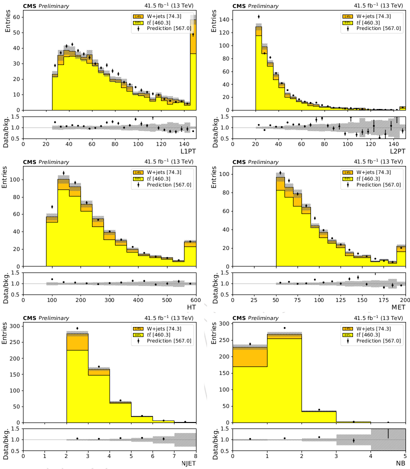
The prediction of events with non-prompt leptons in the signal region is computed by selecting events that pass the signal region selection except that of the three highest $p_T$ leptons, at most one passes the tight selection while the others pass the loose selection. These events are then weighted multiplicatively by a transfer factor, $\mathrm{tf} = \mathrm{fr}(p_T^\mathrm{cc}, \eta, \mathrm{flav}) / (1-\mathrm{fr}(pT^\mathrm{cc}, \eta, \mathrm{flav}))$ for each loose lepton. The transfer factor is derived as follows: \begin{align*} \mathrm{fr} &= \frac{N\mathrm{t}}{N\mathrm{l}} \ \mathrm{fr} &= \frac{N\mathrm{t}}{N\mathrm{t} + N\mathrm{l!t}} \ N\mathrm{t} &= N\mathrm{l!t} \frac{\mathrm{fr}}{1-\mathrm{fr}} \end{align*} where $N\mathrm{t}$, $N\mathrm{l}$, $N_\mathrm{l!t}$ are the number of tight, loose, and loose-not-tight leptons, respectively.

The prediction can then be compared with simulation in the application region to validate the method. This is done by comparing the quantity and analysis quantity distributions of the data-driven prediction to simulated events from processes that are most likely to enter the signal region through fake leptons, $t\bar{t}$ and $W$+Jets. [@Fig:fake_rate_validation] shows a comparison between the prediction from simulation and from the fake rate method. The predictions from the data-driven and simulated estimates are generally within 30% agreement of each other.

{#fig:fake_rate_validation}

Systematic Uncertainties

Systematic uncertainties originate from experimental or theoretical sources and generally cannot be reduced simply by collecting more data, but can be reduced with refined analysis techniques, precision measurements of the underlying processes, or upgraded detecting equipment. The main experimental uncertainties are:

Integrated luminosity: The integrated luminosity is measured using the pixel counting method and is calibrated via the use of van der Meer scans [@LumiMeasurement]. Over Run 2, the total integrated luminosity has an associated uncertainty of 2.3-2.5%.
Jet Energy: Jet energy is subject to a series of corrections to adjust the raw energy readings from the detector to values that more accurately represent the jet's energy[@1607.03663]. One of these corrections, the jet energy scale (JES) a has an associated uncertainty from 1-8% depending on the transverse momentum and pseudorapidity of the jet. The impact of this uncertainty is assessed by shifting the jet energy correction for each jet up and down by one standard deviation before the calculation of all dependent kinematic quantities, $N_\mathrm{jet}$, $HT$, $N\mathrm{b jet}$, and $E!!/_T$. These uncertainties are propagated into these dependent quantities. Most signal regions show yield variations of 8% when the JES is varied by one standard deviation. The jet energy resolution (JER) is considered as well for the simulated backgrounds and signals. The effect of varying jet energy within their resolution on the event counts in the signal region bins is assessed in the same manner as the JES uncertainty.
B-tagging: The efficiency of identifying jets from bottom quarks is different between simulation and data. A scale factor proportional to is applied to simulated events to account for this. The scale factor has an associated systematic uncertainty The varying the scale factor within this uncertainty results in a change in the $t\bar{t}W$ and $t\bar{t}H$ yields in the baseline selection of roughly 8%, and about 6% for $t\bar{t}Z$.
Lepton Efficiency: Lepton efficiency scale factors [@SUSLeptonSF], which account for differences in the efficiency of the reconstruction algorithm for recorded data and simulation, are applied to all simulated events. They result in event weight uncertainties of approximately 2-3% per muon in event and 3-5% per electron in event.
ISR/FSR Reweighting As previously discussed, $t\bar{t}W$ and $t\bar{t}Z$ events are reweighted to correct the distribution of ISR/FSR jets in simulated $t\bar{t}W$ and $t\bar{t}Z$ events to the measured distribution in data. An uncertainty equivalent to 50% of the reweighting factor is associated with this procedure. For 2016 data, the reweighting factor was found to be as low as 0.77, resulting in an uncertainty of 15% on the background prediction in the highest $N_\mathrm{jets}$ signal regions. In 2017 and 2018, the reweighting factor is as large as 1.4, resulting in a similar uncertainty to 2016.
Data-driven background estimations: The non-prompt and charge-misidentification backgrounds estimates have an associated Poisson uncertainty based on the number of application region events used to create the estimate, and this number of events varies dramatically across the individual signal regions. Together with the uncertainties on the fake rate and charge-misidentification rate, this Poisson uncertainty compose the systematic uncertainty on the background estimate. In addition, there is an overall normalization uncertainty applied to the non-prompt background estimate of 30% based on a comparison between the fake estimation described here and an alternative method where the measurement of the fake rate is done "in-situ" in the baseline region[@iso_tuning]. This uncertainty is increased to 60% for electrons with $p_T > 50$ GeV to account for discrepancies in the closure test for those electrons observed in both methods.

Systematic uncertainty also arises from the finite size of simulated data sets. This is handled using the Barlow-Beeston method[@BarlowBeestonMC] within the framework of the Higgs Combine tool. The method accounts for the finite precision and associated uncertainties that arise when making estimations with Monte Carlo methods, and is used to handle both the simulated data and the data driven background estimates' statistical uncertainty.

Signal Extraction and Results {#sec:results}

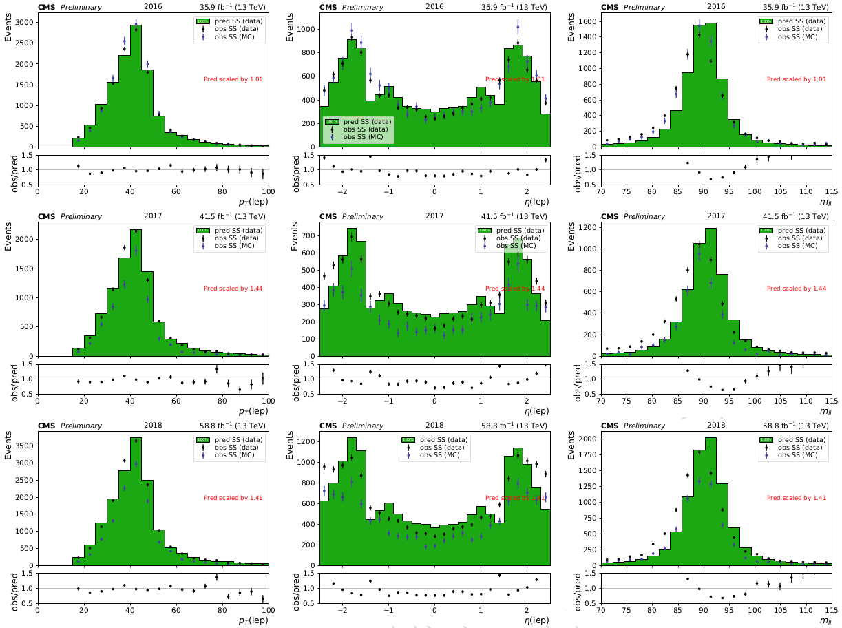
The purpose of this analysis is to search for the presence of $t\bar{t}t\bar{t}$ events within recorded events that fall within the signal regions. To that end, a binned maximum likelihood fit is performed over the signal and control regions using the Higgs Combine tool[@CombineTool]. The input to the fitting procedure are the number of predicted signal and background events in the control and signal regions as well as the observed number of events. The predicted and measured number of events is shown in the top row of [@fig:prefit_postfit]. The maximum likelihood is found by varying the total number of events from each process where the variation is constrained by the normalization uncertainty on that process. The fit also allows bin-to-bin migration of events constrained by the shape uncertainties for each bin. Additional details on how the fit is performed can be found in [@CombineTool] and more information on the specifics of the fit for this analysis and checks that were done to ensure the fit behaves properly can be found in the analysis documentation[@CMSFT2019]. The post-fit distributions are shown in the bottom row of [@fig:prefit_postfit]. Normalization and shape parameters are changed from their a priori values by the fit. These changes are referred to as pulls and are shown in [@fig:impacts].

{#fig:impacts width=100%}

Using the cut-based signal and control region definitions, the expected (observed) significance is 1.7 (2.5) standard deviations in excess of the background prediction, and for the BDT-based regions it is 2.6 (2.7) standard deviations. The observed (expected) 95% confidence level upper limit on the $t\bar{t}t\bar{t}$ production cross section is 20.04 ($9.35{-2.88}^{+4.29}$) fb for the cut-based analysis and 22.51 ($8.46^{+3.91}{-2.57}$) fb for the BDT-based analysis. This is computed using the modified $\mathrm{CL}\mathrm{S}$ criterion [@Junk1999][@Read2002], with the profile likelihood ratio test statistic and asymptotic approximation[@Cowan2011]. Adding the $t\bar{t}t\bar{t}$ prediction into the fit allows for a measurement of its cross section. This is found to be $9.4^{+6.2}{-5.6}$ fb for the cut based analysis and $12.6^{+5.8}{-5.2}$ fb for the BDT-based analysis. Both measurements are consistent with the SM prediction of $12.0^{+2.2}{-2.5}$ fb at NLO. Due to its superior sensitivity, the BDT-based result is taken as the primary measurement of this analysis and is what is used in the interpretations of the result.

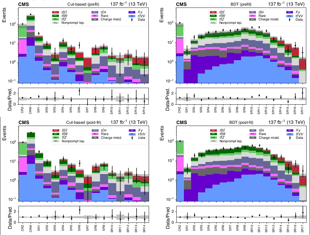{#fig:prefit_postfit width=99%}

Interpretations

The results of this analysis can be interpreted as constraints on other interesting aspects of physics. Considered here are the top quark's Yukawa coupling to the SM Higgs boson, and the Type-II Two Higgs Doublet Model(2HDM).

Top Yukawa Coupling {#sec:top_yukawa}

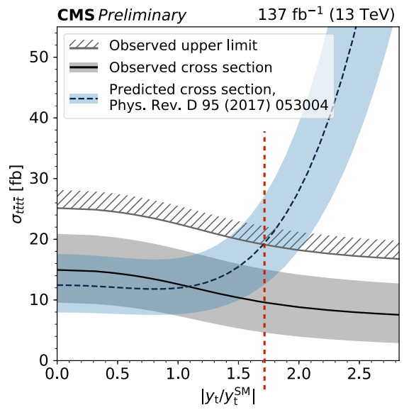
Standard Model production of four top quarks includes Feynman diagrams with an off-shell Higgs boson mediating the interaction (rightmost diagram of [@fig:ft_prod_feyn]). The amplitude of these diagrams is proportional to $y_t^2$. This contributions of these diagrams are added to those of diagrams with no Higgs bosons and squared to give the four top quark production cross section the following dependence on $yt$[@TopYukawaTTTT]. $$ \sigma\left(t\bar{t}t\bar{t}\right) = \sigma{g+Z/\gamma} + k_t^4 \sigma_H + kt^2 \sigma\mathrm{int} $$ where $kt$ is the ratio of the top quark Yukawa coupling to its SM value. The three terms correspond to the no-Higgs contribution ($\sigma{g+Z/\gamma}$), the Higgs contribution ($\sigmaH$), and the interference between the two processes ($\sigma\mathrm{int}$). These terms have been calculated at LO. They are: \begin{align} \sigma_{g+Z/\gamma} =& 9.997 \ \sigmaH =& 1.167 \ \sigma\mathrm{int} =& -1.547 \ \end{align} These terms are calculated at LO, but because the NLO correction to the $t\bar{t}t\bar{t}$ cross section is significant, a correction factor $\sigma{t\bar{t}t\bar{t}}^\mathrm{NLO}/\sigma{t\bar{t}t\bar{t}}^\mathrm{LO}$ is applied to scale the factors to NLO. This results in an NLO cross section of $12.2^{+5.0}_{-4.4}$ fb at $kt=1$, consistent with the full NLO calculation of $11.97^{+2.15}{-2.51}$ fb. This procedure yields the cross section's dependence upon $k_t$ that includes NLO corrections. Another consideration is that $t\bar{t}H$ ($H$ on shell) is a non-negligible background that also scales with $yt$, since $\sigma{t\bar{t}H} \propto \left(y_t / y_t^\mathrm{SM}\right)^2$. Therefore, the limit on the $t\bar{t}t\bar{t}$ cross section decreases as $y_t/y_t^\mathrm{SM}$ grows since the larger $t\bar{t}H$ contribution accounts for a larger proportion of the observed excess. [@Fig:top_yukawa] shows the measured $t\bar{t}t\bar{t}$ cross section as well as its 95% confidence level upper limit and the theoretical prediction of the cross section versus $k_t$. Comparing the observed upper limit with the central value of the theoretical prediction, we claim a limit of $|y_t/y_t^\mathrm{SM}| < 1.7$.

{#fig:top_yukawa width=70%}

Type-II Two Higgs Doublet

As discussed in chapter 2, the Higgs field is introduced as a doublet of complex scalar fields. An interesting Beyond the Standard Model (BSM) theory involves adding an additional doublet. Theories based on this addition are called Two Higgs Doublet Models (2HDM)[@Gaemers:1984sj;@Branco:2011iw]. This increases the number of "Higgs" particles from one to five. These include two neutral scalar CP-even particles, h and H, where conventionally h is taken as the lighter of the two. There is also a neutral pseudoscalar, $A$, and a charged scalar, $\mathrm{H}^\pm$. This following discussion examines how this analyses can be used to set constraints on the new neutral Higgs particles. Keep in mind that notation has changed slightly. Previously, $H$ was the SM Higgs boson, but in this section $h$ is the SM Higgs boson and $H$ is the additional scalar in the 2HDM model.

The 2HDM model contains two parameters that will be used in this interpretation: $\alpha$ which is the angle that diagonalizes the mass-squared matrix of the scalar particles, and $\beta$ which is the angle that diagonalizes the mass-squared matrix of the charged scalars and the pseudoscalar[@Branco:2011iw]. The two parameters, $\alpha$ and $\beta$ then determine the interactions between the various Higgs particles and the vector bosons as well as the fermions, given the fermions' masses. For this interpretation, 2HDM models of Type II are considered, in which the additional Higgs particles couple strongly to the top quark. In this case, one can impose the "alignment limit", $\sin\left(\beta - \alpha\right) \rightarrow 0$, forcing the lighter of the two CP even Higgs bosons, h, to have couplings exactly like the SM Higgs boson, while the couplings of H and A to the SM vector bosons vanish. In this limit, production of H and A is predominantly through gluon fusion.

{#fig:2hdm_diagrams width=99%}

The strategy of this interpretation is to use the same-sign lepton pair final state of the processes shown in [@fig:2hdm_diagrams] to place limits on their cumulative cross section, treating $t\bar{t}t\bar{t}$ as a background with its SM predicted cross section. This is done by simulating events and calculating cross sections for the 2HDM processes using the 2HDMtII_NLO MadGraph model[@Craig:2016ygr] on a grid of points made by varying the mediating particles' masses and $\tan\beta$. The resulting cross section predictions are shown in [@fig:2hdm_cross_sections].

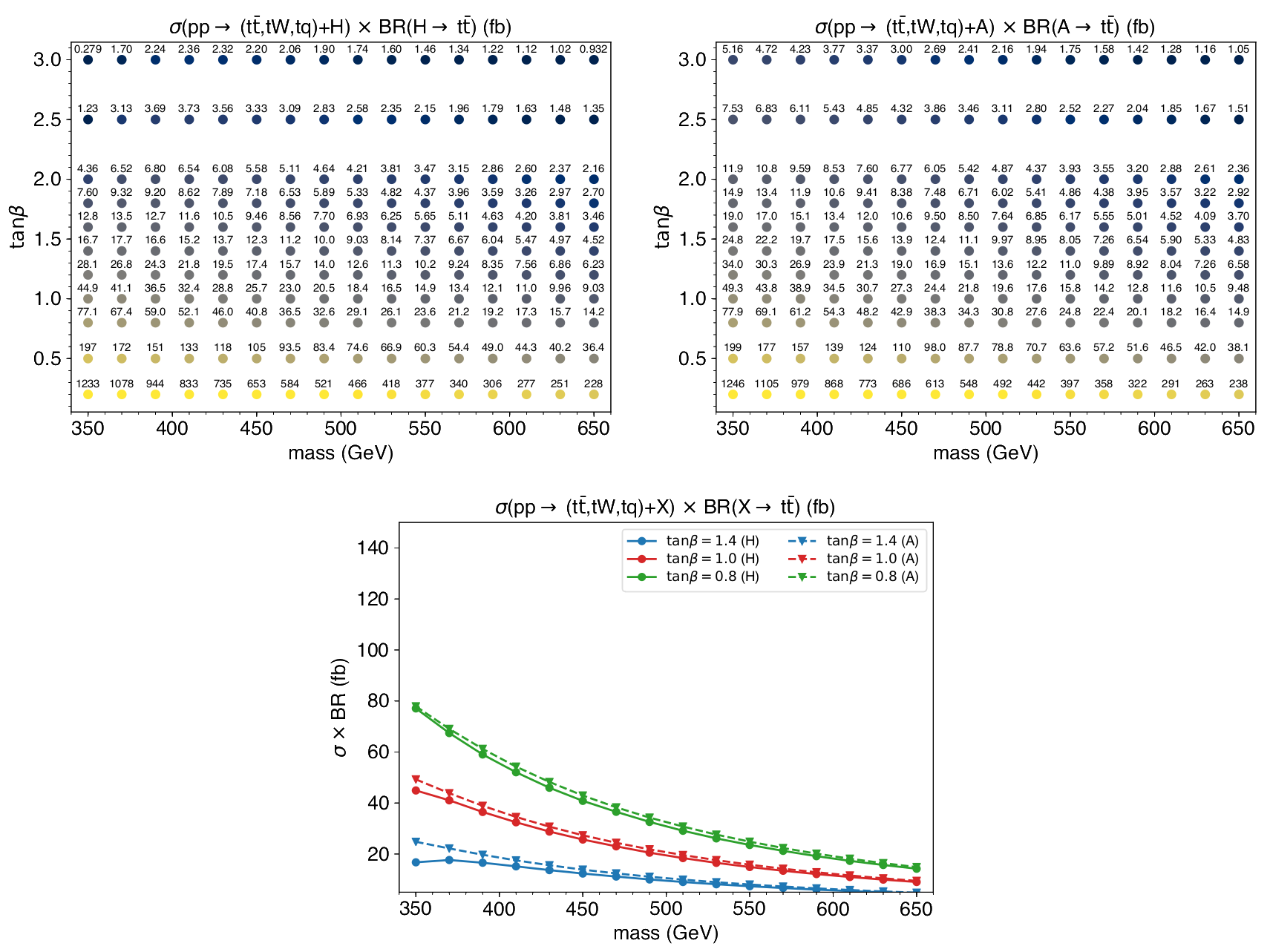{#fig:2hdm_cross_sections width=100%}

In general, the kinematic distributions of events originating from a scalar or pseudoscalar mediator will be different. This means that the acceptance, or proportion of events that lie within the signal regions, will be different between the two processes. This would need to be accounted for when placing limits. However, [@Fig:2hdm_kinematics] shows a comparison of analysis level observables for the two processes, and the two distributions are similar. In particular, the BDT discriminant distribution has a Kolmogovor-Smirnov test metric of 0.8, indicating consistency within statistical limits. This implies that the acceptance difference between the two processes is small enough to be ignored. For this reason, only scalar samples are used for both processes, and the pseudoscalar results are obtained by scaling the cross section appropriately.

{#fig:2hdm_kinematics}

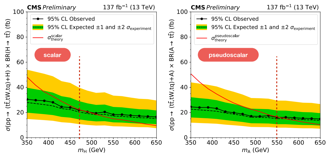
Limits are calculated by placing simulated events from either the $H$-mediated processes or the $A$-mediated diagrams into the BDT-based signal regions as previously defined. A fit is performed similarly to the $t\bar{t}t\bar{t}$ measurement except for that the Standard Model four top quark production is treated as a background and it's cross section is treated as a nuisance parameter. This is done for each combination of mediator mass and $\tan\beta$. Points where the 95% CL limit on the cross section is smaller than the predicted cross section are considered excluded. [@Fig:2hdm_2dexclusions] shows the resulting exclusions. At $\tan\beta=1$, scalar (pseudoscalar) heavy bosons are excluded up to 470 (550) GeV ([@fig:2hdm_exclusions]).

{#fig:2hdm_2dexclusions}

{#fig:2hdm_exclusions}

05_tttt_measurement.md 65 KB Permalink Histórico Raw