thesis/content/04_simulation_and_reconstruction.md

---

title: Event Simulation and Reconstruction ...

An essential aspect of particle physics experiments is the ability to accurately infer the types of particles and their kinematic properties in each event from the raw detector readings. This process is called event reconstruction. To achieve this, sophisticated algorithms are developed to correlate readings within and across subdetectors. The development of these algorithms is guided by an accurate simulation of the detector response to simulated collisions. Simulation is also employed in the interpretation of physics measurements by providing predictions for the rate and kinematics of physics processes of interest. Disagreement between experimental observation and predictions made in this way can be an indication of new physics, but can also point out mis-modeling of the detector, the physics process, or simply bugs in any part of the software chain. Therefore, rigorous examination and crosschecks must be applied to instill confidence in the accuracy of the simulation.

Event Simulation

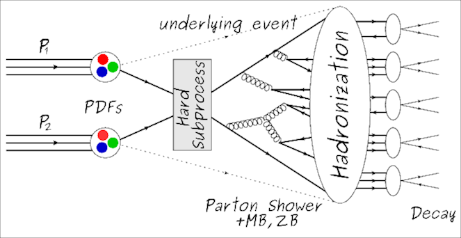
Event generator software is used to simulate the initial hard-scatter of partons from the colliding protons. The software used by LHC experiments implements sophisticated Monte-Carlo (MC) techniques to both calculate cross-sections for SM and certain BSM processes, and to generate samples of events that can be compared with real data. The generation of events can be broken down into four distinct stages.

1. Hard Scatter: This step uses the parton distribution functions (PDFs). The PDFs are effectively the probability distributions of the proton's different constituent particles to carry a certain fraction of its energy. Then the rules of perturbative quantum field theory are applied to create a set of Feynman diagrams for the process under consideration (e.g. $gg\rightarrow t\bar{t}$). The integrals encoded by these diagrams are then calculated using Monte-Carlo methods to produce a cross section and set of events with the output particles having the correct angular and momenta distributions up to some order of perturbation theory.
2. Hadronization and Fragmentation: The particles produced by the hard scatter step are often not the particles that will be observed by the detector. For example, quarks will generally hadronize and form jets. Colored and charged particles can radiate gluons and photons, respectively. The partons of the interacting protons not directly involved in the hard scatter will generally also fragment and result in additional particles. These are referred to as the "underlying event".
3. Mixing: Each bunch-crossing has many additional, though generally with low momentum transfer, proton-proton interactions that also create particles. These extra collisions are referred to as "pileup interactions". Many of these events are simulated separately and then "mixed" with the hard scatter event to produce a realistic collision.
4. Detector Response: At this stage, the collection of particles in the event are the ones that will interact with the detector materials. A detailed model of CMS is used with GEANT4[@Agostinelli2003] to simulate interactions with detector materials. This includes bremsstrahlung radiation, electromagnetic and hadronic showers, and decays of unstable hadrons in-flight. The result of this simulation is a set of readings in detector readout electronics that can then be fed into the same reconstruction algorithms that are used for real data.

{#fig:generator width=70%}

Event Reconstruction

The strategy that CMS uses to reconstruct particles is referred to as "Particle Flow" (PF)[@CMS-PRF-14-001]. PF attempts to identify every particle in the event. This approach requires a very highly granular detector to separate out nearby particles. High granularity becomes particularly important in the process of reconstructing jets which can consist of many closely spaced particles. The calorimetry system can be used to measure the jet energy, but in combination with the tracker to measure the momentum of the charged components of the jet, the precision of measurement can be improved dramatically. The key, then, to PF reconstruction is to be able to link together hits in the different subdetectors to increase reconstruction effectiveness, while at the same time avoiding assigning any particular detector signal to multiple particles.

Before the readings in individual subdetectors can be linked together, their raw hit data must be processed into higher level objects. For the tracker, the first step is to combine hits in adjacent pixels together into groups whose charges presumably originated from a single particle. This process is called clustering. The next step involves finding the sets of clusters across layers that that can be strung together to form the track of a particle. The generic algorithm for this is called Combinatorial Track Finding (CTF)[@Billoir1990]. The first step in CTF is finding pairs, triplets, or in the case of the Phase I upgrade, quadruplets, of clusters in the pixel detector that are consistent with a track originating from the luminous region of CMS. This gives an initial estimate of the particle's charge and momentum, along with associated uncertainties. A statistical model augmented with physical rules known as a Kalman Filter is employed to extrapolate this "seed" through the rest of the tracker, attaching more clusters as the extrapolation moves through the tracker. A helical best-fit is done on the final collection of clusters. The quality of this fit, along with other quality metrics such as the number of layers with missing clusters, is used to decide if this track is to be kept for further processing. This procedure is performed in several iterations, starting with very stringent matching requirements to identify the "easy" to reconstruct particles (generally isolated, with high momentum). Clusters from earlier iterations are removed so that subsequent iterations with looser matching requirements do not suffer from a prohibitively large number of combinations. This approach is also applied to the muon system to build muon tracks.

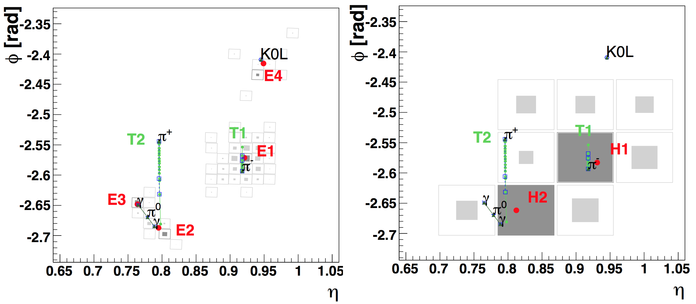
In the calorimeters, hits in individual ECAL crystals or HCAL towers are grouped to form clusters. This clustering is performed by first finding local maxima in the energy deposition across the calorimeter. These maxima are called seeds. Crystals/towers adjacent to the seeds with energy above a certain threshold are then grouped with the seed, forming a cluster. In a crowded event, it is possible for different clusters to overlap. In this case, a specialized algorithm is employed to compute the sharing of energy between the clusters. An example event demonstrating this is shown in [@fig:cal_clusters].

{#fig:cal_clusters}

The final step in the PF algorithm is to link together the building blocks from the four subdetectors: tracks from the tracker and muon system, and ECAL and HCAL clusters. Tracks from the tracker are matched with clusters by extrapolating the helical track to the depth in the calorimeter where the shower is expected to have started. If this position lies within a cluster, the track is linked with it. Bremsstrahlung photons from electrons are accounted for by looking for additional ECAL deposits that align with the tangent of the track at its intersection with each of the tracker layers. If such deposits exist, they are linked with the track also. Clusters in the ECAL and HCAL, as well as the ES and ECAL, can be linked if the ECAL(ES) cluster lies within the boundaries of an HCAL(ECAL) cluster in the $\eta-\phi$ plane. Finally, if a combined fit between a tracker track and a muon system track results in a sufficiently small $\chi^2$, the two tracks are linked together.

The PF particle collection is created from a set of linked blocks based on which subdetectors contributed hits to it. The options are:

• charged hadron: a tracker track and HCAL cluster
• neutral hadron: an HCAL cluster with no tracker track
• electron: a tracker track and ECAL cluster
• photon: an ECAL cluster with no tracker track
• muon: a tracker track matched with a muon system track

The output of the PF algorithm is a collection of reconstructed particles and their momenta. This information can then be fed into higher-level algorithms to reconstruct jets, including jet flavor, and transverse momentum imbalance.

Jet Reconstruction

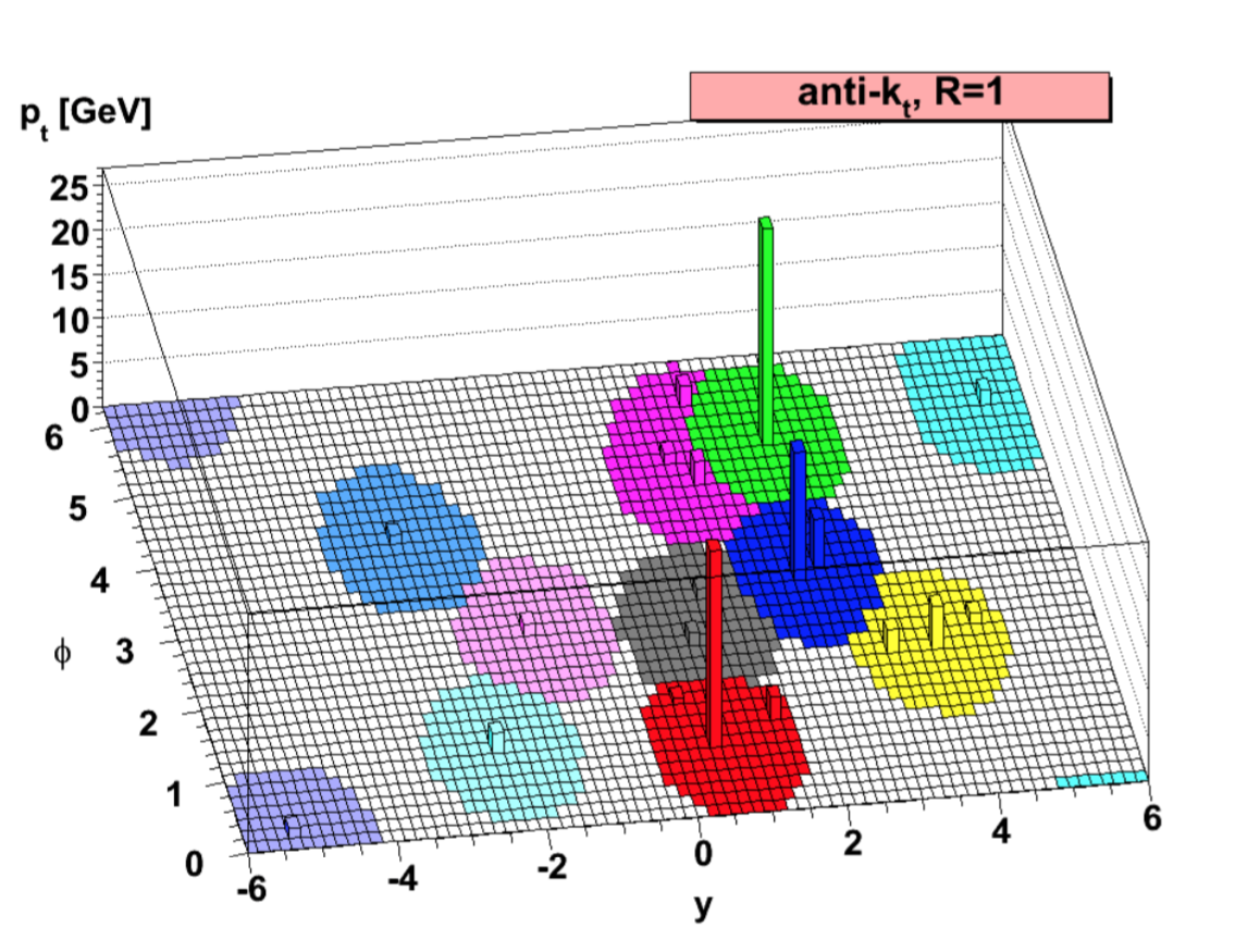
As mentioned in chapter 2, highly energetic quarks produced in LHC collisions fragment to produce a spray of collimated particles referred to as a jet. Jets are constructed from PF particles using the anti-$k_T$ clustering algorithm[@Cacciari2008]. The anti-$kT$ algorithm works as follows. For each input object k and for each pair of objects ($i$, $j$), a beam-distance $d{kB}$ and a distance $d_ij$ is calculated. They are defined as \begin{align*}

d_{kB} &= 1/\left( p_{T}^k \right)^2 \\
d_{ij} &= \mathrm{min}\left( \left( p_{T}^i \right)^2, \left( p_{T}^j \right)^2 \right) \frac{\Delta R_{ij}^2}{R^2}

\end{align*} where R is a tunable parameter setting the granularity of the jet reconstruction, but has typical values are around 0.4-0.5. The smallest $d{ij}$ is compared to the smallest $d{kB}$. If it smaller, the objects $i$ and $j$ are combined into a new object with momentum $p = p_i + p_j$, otherwise the object $k$ is considered as a jet and removed from the collection of objects. This procedure iterates until all objects have been removed. This algorithm leads to jets that have a circular shape as shown in [@fig:anti_kt].

{#fig:anti_kt}

Bottom Quark Jet Identification

Bottom quarks have very small CKM couplings to the other quarks which decreases their decay rate to lighter quarks. This leads to bottom flavored hadrons produced in collisions traveling a measurable distance, typically on the order of a few millimeters, from the primary interaction before decaying. The secondary vertex defined by this decay point is a signature of bottom quarks. Jets resulting from bottom quarks also contain on average more particles than jets from lighter quarks due to the bottom quark's higher mass. CMS deploys a dedicated algorithm[@CMS-DP-2017-005] to combine information related to these qualities from the particles reconstructed from PF to identify bottom quarks. This procedure is referred to as b-tagging.

Missing Transverse Momentum

In hadron collisions the longitudinal momentum of the colliding partons is unknown. However, the transverse momentum is zero[^1]. This fact can be used to infer the presence of particles that are invisible to the CMS detector. In the SM these are neutrinos, but theories beyond the Standard Model predict other particles that will not be seen such as dark matter particles. The metric that is used to make this inference is the missing transverse momentum, $p!!!/_T$. This is calculated by taking the negative of the vector sum of the transverse momenta of all observed particles. For events that produce no undetected particles, this sum should be very close to zero, otherwise the undetected particle(s) will leave an imbalance. The magnitude of the missing transverse momentum is called the missing transverse energy, $E!!!!/_T$.

[^1]: Technically the partons have some initial transverse momentum due to beam dispersion, and momenta of the parton within the rest-frame of the proton, but these are tiny.

Optimization of Electron Seed Production

Like the tracking algorithm described above, the reconstruction of electrons begins with the creation of electron seeds. Part of the research for this dissertation involved the tuning of the algorithm that builds these seeds. This section discusses that work.

The construction of electron seeds consists of linking together tracker seeds with ECAL Superclusters (SC). These tracker seeds originate through the same method as the seeds used in PF tracking. They are collections of pixel clusters across layers in the pixel detector that are consistent with a particle originating in the luminous region. A SC is a set of nearby ECAL crystals whose energy distribution passes certain criteria to allow them to be grouped together. The procedure for matching tracker seeds with SCs is as follows:

1. Use the SC energy and position with the position of the beam-spot to make a track hypothesis for both positive and negative charge. [@Fig:seed_match] shows one possible charge hypothesis.
2. Project that track onto the layer of the innermost hit in the tracker seed under consideration. Require that the hit position and track projection are within a certain ($\delta \phi$, $\delta R/z$) window of each other. The orientation of the layers of the tracker dictates that $z$ be used for BPIX and $R$ for FPIX. Because the initial track hypothesis uses the beam spot, which is elongated several centimeters in z, this initial matching uses a large $\delta R/z$ window.
3. Create a new track hypothesis using the beam spot and the first hit position with the energy of the SC. The $z$ coordinate of the beam spot position is calculated by projecting a line from the SC through the first matched hit to the point of closest approach with the z-axis.
4. Project the new track out onto the layers of successive hits in the tracker seed. Again, require that the projected position and the hit match within a certain window.
5. Quit either when a hit fails to match or when all hits have been matched.

If a tracker seed has enough matching hits it is paired with the SC, and they are passed together for full electron tracking. This involves the use of a modified Kalman Filter known as a Gaussian Sum Filter to propagate the initial track through the rest of the tracker. These "GSF electrons" continue on to several more filters and corrections before they are used in physics analyses.

Electron seeds created through this procedure are referred to as "ECAL-driven". There are also "tracker-driven" electron seeds which are not matched with ECAL SCs, and proceed through the GSF tracking algorithm based on tracker information alone. After the track has been reconstructed, it may then be matched with a SC. The tracker-driven seeds help to compensate for inefficiencies coming from the ECAL-driven matching procedure. In the end, the ECAL-driven and tracker-driven electron collections are merged to produce a single collection of electron candidates.

{#fig:seed_match}

This general approach was developed during early CMS operation, but the installment of the Phase I pixel detector motivated a re-write of the underlying algorithm to handle the additional layers. The new implementation was designed to be more flexible, allowing for a variable requirement on the number of matched hits, a significant change from the previous algorithm which would only match two hits. Work was done to optimize this new hit-matching algorithm for the new pixel detector. In particular, the $\delta \phi$ and $\delta R/z$[^2] windows were tuned to maximize efficiency while also keeping the number of spurious electron seeds at a minimum.

[^2]: $R/z$ should be understood as either $R$ or $z$ based on whether hits in the barrel or endcap are being considered, not as a ratio.

The size of these matching windows is defined parametrically in terms of the transverse energy($E_T$) of the SC. The transverse energy is $E\cos\theta$, where $E$ is the energy of the SC. The function for determining the window size is

$$ \delta(E_T)= \begin{cases}

E_T^{\mathrm{high}} ,& E_T > E_T^{\mathrm{thresh}} \\
E_T^{\mathrm{high} } + s(E_T - E_T^{\mathrm{thresh}}) ,& \mathrm{otherwise}

\end{cases} $$

Normally, $s$ is negative which means that the cut becomes tighter with higher $E_T$ until $E_T^{\mathrm{thresh}}$ where it becomes a constant. So the optimization was to $E_T^{\mathrm{high}}$, $E_T^{\mathrm{thresh}}$, and $s$. The challenge to performing a rigorous optimization of these parameters is that they are individually defined for the first, second, and any additional matched hits and also separately for $\phi$ and in $R/z$, meaning that the optimization would have to be performed in many dimensions. In addition, the figure of merit for the optimization is difficult to clearly define since a balance must be struck between electron reconstruction efficiency and the purity of the set of reconstructed electrons. Given these challenges, a more ad-hoc approach was developed. The approach consisted of first acquiring two samples of simulated data: A simulated sample of $t\bar{t}$ events with many jets containing photons and charged hadrons capable of faking electrons, as well as genuine electrons from W boson decays, and a sample of simulated $Z\rightarrow e^+e^-$ events with many genuine electrons and relatively few electron faking objects. The next step is to define efficiency and purity metrics. Because this is simulated data, it is possible to perform truth-matching to determine if a reconstructed track originated from an electron or not. A reconstructed electron is considered truth-matched if there is a simulated electron in the event within a cone of $\Delta R<0.2$ centered on the reconstructed electron. Efficiency is then defined as the proportion of simulated electrons that get successfully reconstructed as ECAL-driven GSF tracks, and purity is the proportion of ECAL-driven GSF tracks that resulted from a simulated electron.

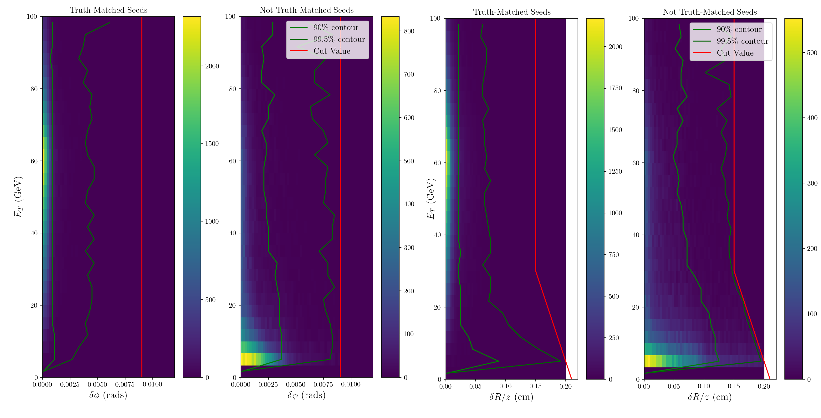
Hit residuals are the $\delta \phi$ and $\delta R/z$ between hits and the projected track in the matching procedure. Understanding the distribution of these residuals will guide the choice of matching windows. The simplest way to study the residuals is to run the hit-matching algorithm with very wide windows to avoid imposing an artificial cutoff on the distributions of the residuals. [@Fig:combined_residuals] shows the distributions of residuals of hits in the innermost barrel layer for truth-matched and non-truth-matched seeds. Also plotted are the contours where 90% or 99.5% of hits are to the left. The residual distributions are very different based on whether the seed was truth-matched or not. Recall that for the first hit, the luminous region is used for one end of the projected track, and since the luminous region is significantly elongated in z, the residuals can be quite large. However, the $\delta \phi$ residuals for truth-matched tracks tend to be tiny (<.5°), while non-truth-matched residuals tend to be larger, especially at low $E_T$.

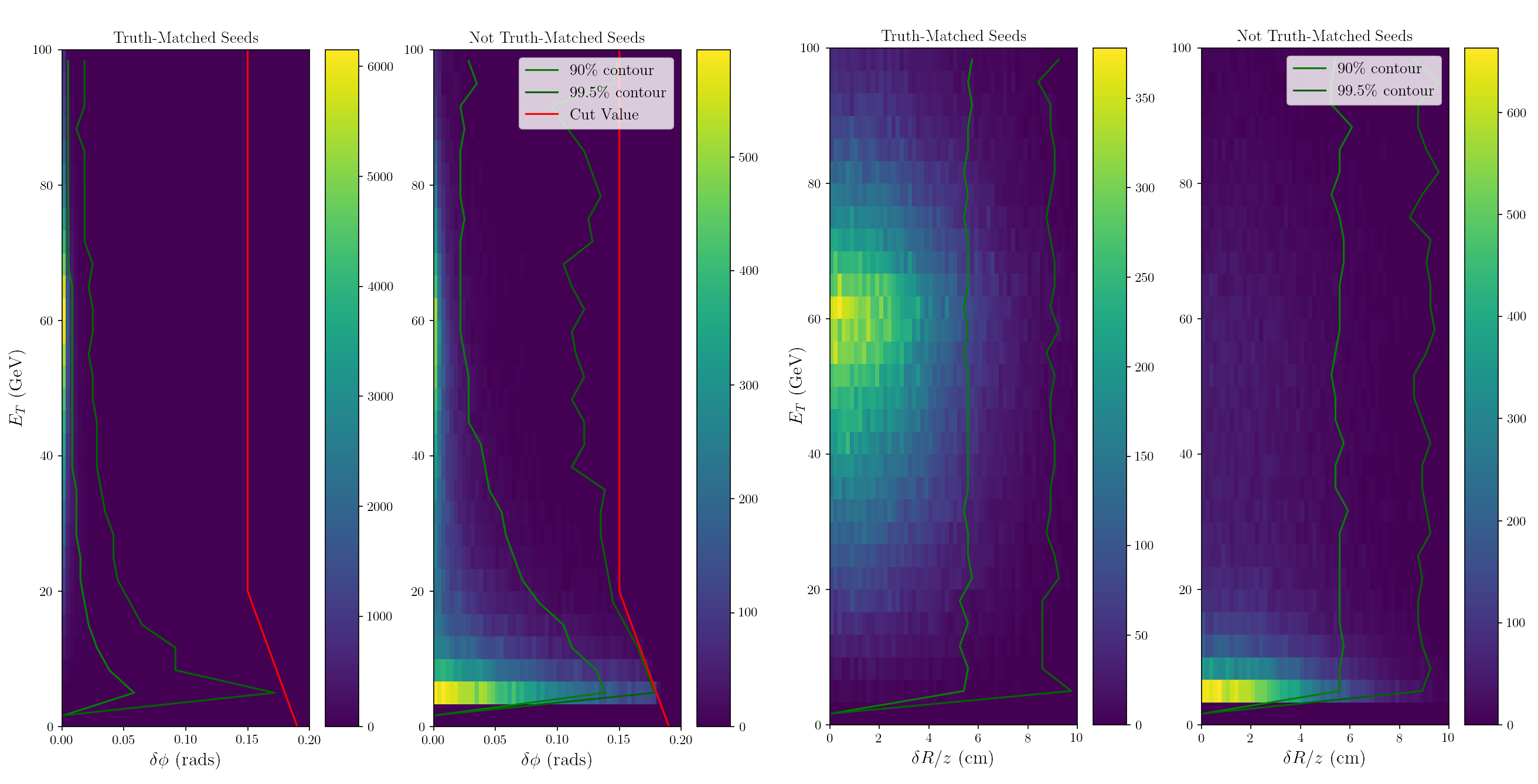{#fig:combined_residuals}

[@Fig:combined_residuals_L2] shows the residuals for the second matched hit for hits in the second barrel layer. After matching the first pixel hit, the projection of the track becomes much more precise, roughly a factor of 20 times smaller for $\delta \phi$ and over 200 times smaller for $\delta z$.

{#fig:combined_residuals_L2}

Guided by these distributions, four sets of windows were designed with varying degrees of restriction. The parameters for these windows are listed in [table @tbl:windows].

		extra-narrow	narrow(default)	wide	extra-wide
Hit 1	$\delta \phi$ : $E_T^\mathrm{high}$	0.025	0.05	0.1	0.15
	$\delta \phi$ : $E_T^\mathrm{thresh}$	20.0	20.0	20.0	20.0
	$\delta \phi$ : $s$	-0.002	-0.002	-0.002	-0.002
	$\delta R/z$ : $E_T^\mathrm{high}$	9999.0	9999.0	9999.0	9999.0
	$\delta R/z$ : $E_T^\mathrm{thresh}$	0.0	0.0	0.0	0.0
	$\delta R/z$ : $s$	0.0	0.0	0.0	0.0
Hit 2	$\delta \phi$ : $E_T^\mathrm{high}$	0.0015	0.003	0.006	0.009
	$\delta \phi$ : $E_T^\mathrm{thresh}$	0.0	0.0	0.0	0.0
	$\delta \phi$ : $s$	0.0	0.0	0.0	0.0
	$\delta R/z$ : $E_T^\mathrm{high}$	0.025	0.05	0.1	0.15
	$\delta R/z$ : $E_T^\mathrm{thresh}$	30.0	30.0	30.0	30.0
	$\delta R/z$ : $s$	-0.002	-0.002	-0.002	-0.002
Hit 3+	$\delta \phi$ : $E_T^\mathrm{high}$	0.0015	0.003	0.006	0.009
	$\delta \phi$ : $E_T^\mathrm{thresh}$	0.0	0.0	0.0	0.0
	$\delta \phi$ : $s$	0.0	0.0	0.0	0.0
	$\delta R/z$ : $E_T^\mathrm{high}$	0.025	0.05	0.1	0.15
	$\delta R/z$ : $E_T^\mathrm{thresh}$	30.0	30.0	30.0	30.0
	$\delta R/z$ : $s$	-0.002	-0.002	-0.002	-0.002

: Parameters for pixel-matching windows. The narrow window was developed for the HLT deployment of the algorithm, and will also be referred to as default, while the extra-narrow, wide, and extra-wide windows are the HLT settings scaled by 0.5, 2, and 3, respectively. Bold numbers indicate parameters that are modified across window settings. {#tbl:windows}

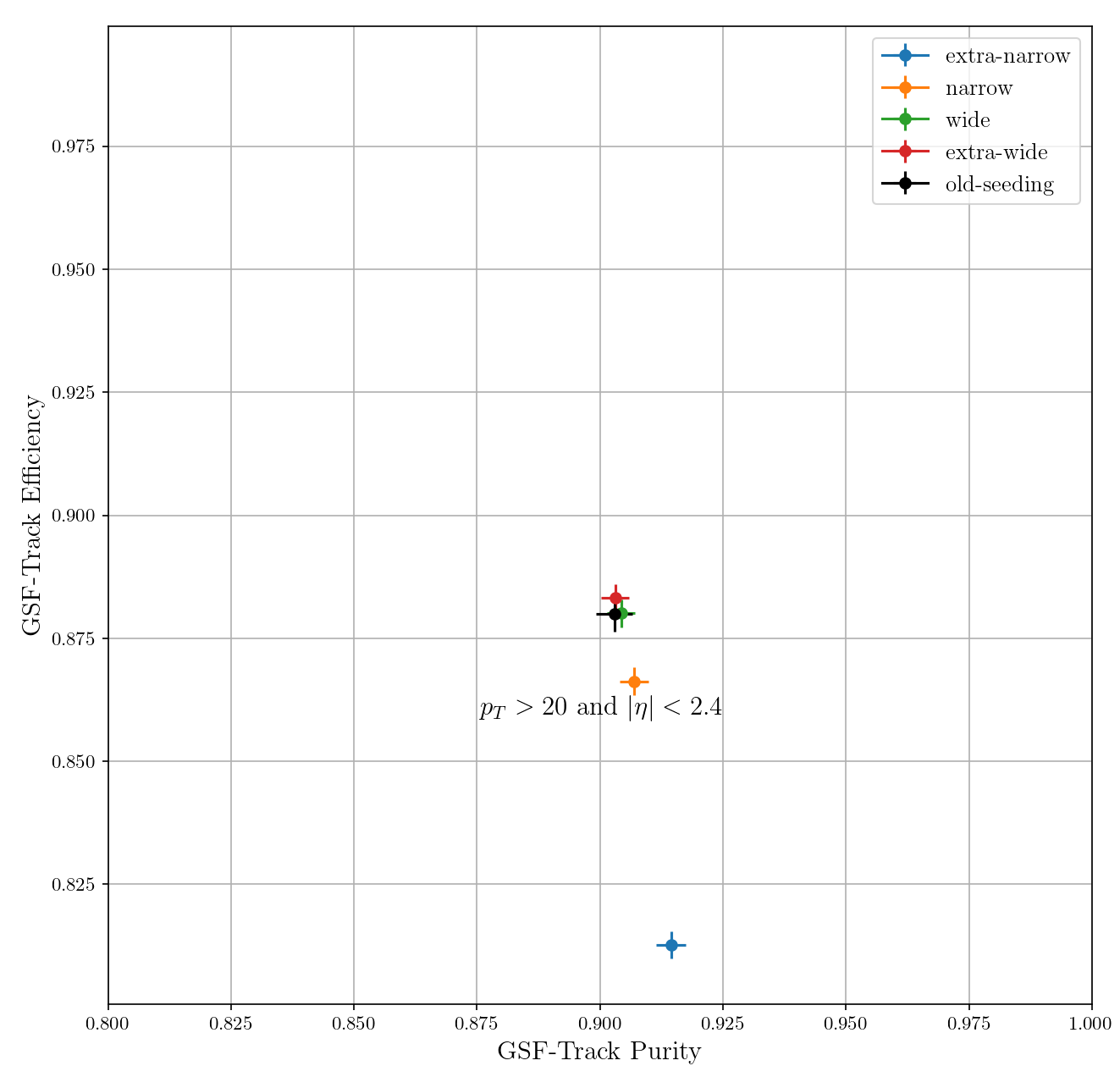
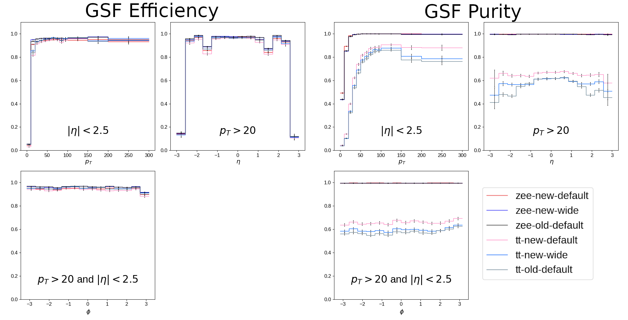
The pixel-matching algorithm was run on simulated data and efficiency and purity were measured, as is plotted in [@fig:gsf_roc]. Of the four working points, extra-narrow was discarded for its distinct drop in efficiency and the extra-wide working point was dropped for being negligibly different from the wide working point. The performance of the remaining two working points on electron candidates using simulated samples of $Z\rightarrow e^+e^-$ and $t\bar{t}$ events are shown in [@fig:gsf_combined]. This figure shows efficiency and purity differentially in $p_T$[^3], $\eta$, and $\phi$ of the GSF tracks that resulted from the pixel-matched seeds. The performance of the algorithm is demonstrated to be as good or better than the original implementation.

[^3]: We use $p_T$ here instead of $E_T$ because these are track kinematics, not SC quantities, although in practice they will be quite similar

{#fig:gsf_roc}

{#fig:gsf_combined}

Another feature of the new algorithm is that on average it produces fewer seeds. In the old algorithm, only pairs of hits are matched. However, the additional layers of the Phase I pixel tracker created tracker seeds with up to four hits making matching only two hits easier and resulting in more electron seeds. The additional seeds created computational issues for HLT, which motivated the rewrite. [@Fig:n_seeds] shows how the number of seeds is reduced by the new algorithm.

{#fig:n_seeds width=80%}

An important feature of the initial implementation was that in the process of matching two hits in the tracker seed, it could skip hits. Hit skipping refers to a feature of the matching algorithm such that if a hit fails to satisfy its prescribed matching criteria, it is skipped and that criteria is instead applied to the next hit in the tracker seed. As long as a sufficient number of hits match, the tracker seed is matched with the SC. The rewrite did not include this feature, and lack of hit-skipping can lead to a loss of efficiency because it is more selective about what seeds get matched with each SC. To avoid this inefficiency, a workaround was introduced.

To understand the workaround, one first has to understand how these tracker seeds are constructed. As mentioned previously, these seeds are normally created through several iterations, starting with quite stringent requirements. Hits that make it into these initial seeds are removed from consideration in subsequent iterations. By removing hits in each iteration, later iterations can have much less stringent requirements on matching hits across layers without creating an unnecessarily large number of tracker seeds. To demonstrate how this is related to hit-skipping, suppose that seeds are generated in three iterations: First, look for quadruplets across four BPIX layers. Second, look for triplets across any combinations of three of the four layers. Finally, look for pairs across combinations of two of the four layers. Let us consider the case where the detector recorded one hit in each BPIX layer and all four hits can match with each other for the purposes of making tracker seeds. The top row of [@fig:hit_skipping] demonstrates how the seeding procedure would normally work. There would be a single quadruplet seed, and no pairs or triplets since all four hits have been removed from consideration in subsequent iterations. This quadruplet is then compared with some SC to make an electron seed. We require that there be three matched hits for triplets and quadruplets, and just two for pairs. During the matching procedure, the hit in BPIX layer 3 (BPIX3) fails to match, however it can be skipped and hit 4 matches. Therefore, the tracker seed matches with the SC and proceeds through the rest of the reconstruction chain. However, if hit-skipping is disabled one gets the situation in the middle row of [@fig:hit_skipping] where the unmatched hit in layer 3 cannot be skipped and as a result only two hits are matched and no electron seed gets produced. The workaround to recover this seed is to disable the removal of hits between tracker seed construction iterations. As a result, many more seeds are created, as shown in the bottom row of [@fig:hit_skipping]. However, the seed (now a triplet) of hits in the first, second, and fourth layers now matches and the electron seed is recovered.

{#fig:hit_skipping width=60%}

From a computational standpoint, this situation is not ideal. Therefore, work was done to add the hit-skipping feature to the new implementation. Adding hit skipping to the new implementation and removing the workaround reduced the number of seeds in $t\bar{t}$ by 41% with the narrow matching window sizes and 36% for the wide windows. Compared to the original pixel-matching implementation, there were also far fewer seeds, dropping from 12.6 on average to 2.5 for the narrow windows and 4.6 for the wide. This is achieved without sacrificing performance in efficiency or purity.