
03_lhc_and_cms_detector.md 24 KB
title: The LHC and CMS Detector ...
Lying buried beneath Geneve, Switzerland and stretching across the border into France is the largest machine ever constructed by mankind. This marvel of physics and engineering is operated by CERN, the European Organization for Nuclear Research[^1]. This machine, the Large Hadron Collider is a circular particle accelerator with a circumference of 28 km that is capable of creating proton-proton collisions with up to 13 TeV of energy in the center-of-mass frame. CERN itself is a huge organization, comprising roughly thirteen thousand people with diverse backgrounds and disciplines. The goal of the LHC and associated experiments is to increase humanity's fundamental understanding of the nature of the Universe. It accomplishes this by studying the unique properties of matter in the extreme conditions created in very high energy particle collisions. These properties are examined by analyzing the data collected by sophisticated particle detectors at several designated points around the LHC ring. The detectors are marvels unto themselves, often designed and operated by collaborations of thousands of physicists and engineers from across the world. The principle detectors on the LHC ring are ALICE, ATLAS, CMS, and LHCb. ATLAS and CMS are general purpose detectors, facilitating a wide range of physics measurements. ALICE specializes in exploring the physics of heavy-ion collisions, exploring the dynamics of the quark-gluon plasma created during collisions of lead or gold ions. LHCb is another specialized detector that focuses on phenomena related to the bottom quark.
[^1]: Acronym derived from the original French: "Conseil Européen pour la Recherche Nucléaire"
The LHC
After initial setbacks in 2008[@quench2008], the LHC began supplying collisions for physics research in 2010 with collision energies of 7 TeV. It operated successfully over the next few years, delivering sufficient high energy collisions to allow for the joint discovery in 2012 by CMS and ATLAS of a new particle with a mass of 125 GeV identified as the Higgs boson[@1207.7214;@1207.7235], as well as a multitude of measurements of SM processes and exclusions of vast swaths of BSM theories. It then underwent an upgrade to increase the center-of-mass energy to 13 TeV, and went on to successfully deliver collisions to CMS over a span of three years from 2016 to 2018.
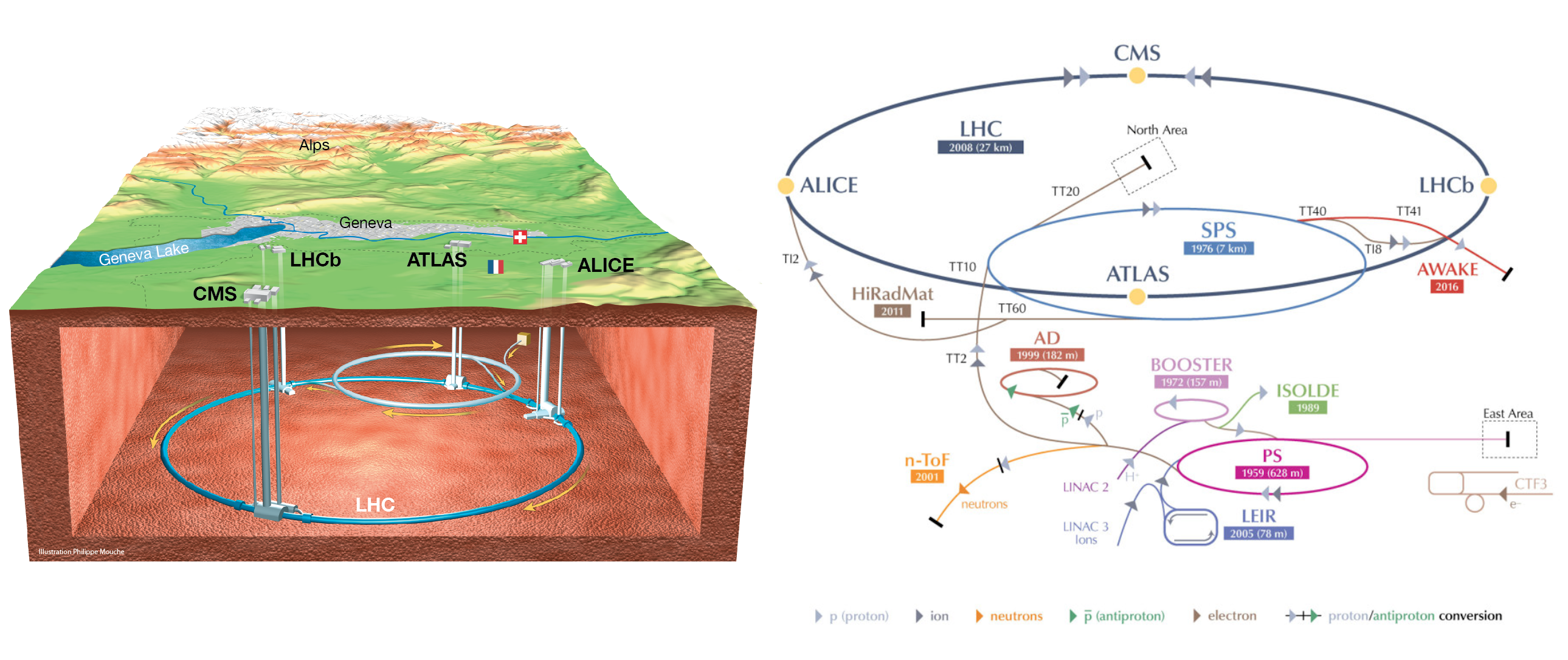
The LHC complex is shown in [@fig:lhc_complex]. Before entering the LHC, protons are collected, bunched, accelerated by several steps. The protons originate as hydrogen atoms that have been ionized by a strong electric field. The $H^+$ ions (i.e. protons) are then accelerated to 50 MeV by the LINAC2 linear accelerator. They are then transferred to the Proton Synchrotron (PS) which further accelerates the protons to 26 GeV. Next, they are injected into the Super Proton Synchrotron (SPS) which pushes their energy to 450 GeV before finally entering the LHC and being pushed to 6.5 TeV. There are two separate injection pathways for injecting protons into the clockwise and the counterclockwise beam channels.
 {#fig:lhc_complex}
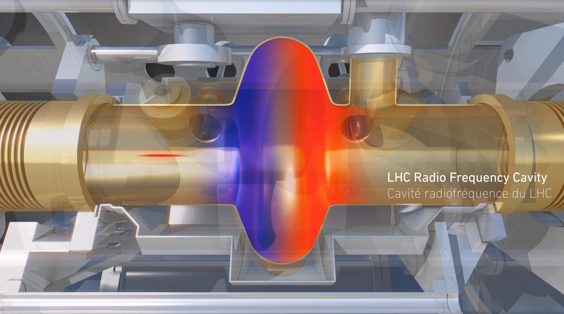
The acceleration of the protons is done with superconducting radio-frequency (RF) cavities ([@fig:rf_cavity]). The LHC has a system of 16 of these cavities concentrated at a single location along the ring. To bend the proton beam around the LHC ring, superconducting dipole magnets are used. [@Fig:lhc_dipole_cartoon] demonstrates how these magnets act to steer the beam. The LHC has 1232 such magnets distributed around eight curved sections of the ring, the curved sections being 2.45 km long each and separated by 545 m long straight sections containing the RF acceleration system, beam dump, and detector halls.
 {#fig:rf_cavity}
 {#fig:lhc_dipole_cartoon}
The beams of protons are not continuous, but are grouped into bunches of roughly 100 billion protons each. Each bunch has a transverse diameter of roughly 1 mm and is approximately 7.5 cm long. The bunches of protons will inevitably have some spread in momentum transverse to the beam direction, exacerbated by the repulsive Coulomb force amongst the protons in each bunch. To account for this, sextupole magnets are employed to condition the beam. As the beam approaches each of the interaction points, quadrupole magnets are used to focus the beam down to having a width of just 16 $\mu \mathrm{m}$ in order to increase the average number of collisions as the opposing beams cross. The number of interactions that occur during each bunch-crossing is tuned to balance maximizing the total number of collisions with what the detector can effectively handle. If there are too many simultaneous interactions in a single bunch crossing, the detector's electronics are at risk of buffer overflows, leading to data loss. It also increases, potentially dramatically, the amount of computing resources that are required to reconstruct each event. The reconstruction of charged particle paths through the detector, or tracks, in particular can become prohibitively expensive as the number of interactions grows. The instantaneous luminosity, directly related to the number of interactions per bunch-crossing, can be calculated using
$$L = fn\frac{N^2}{4\pi\sigma^2}$$ {#eq:inst_lumi}
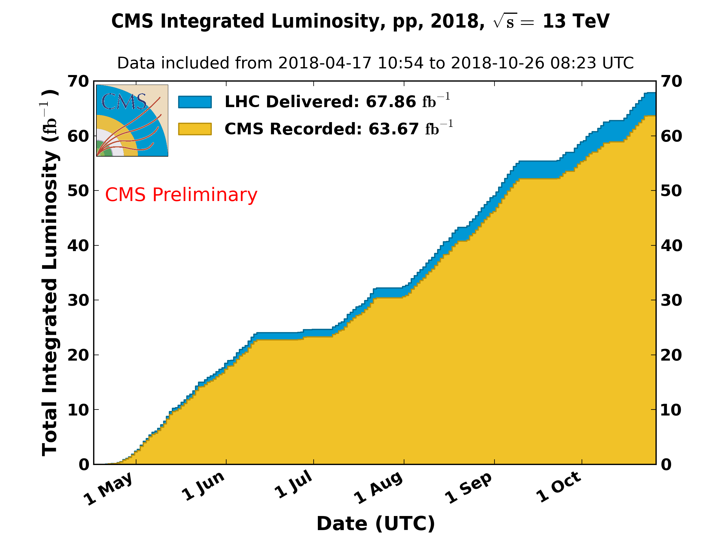
In the above equation, $f$ is the orbit frequency of bunches around the LHC ring, $n$ is the number of bunches per beam. So, $2fn$ is effectively the bunch-crossing frequency[^2]. $N$ is the number of protons per bunch and $\sigma$ is the Gaussian width of the beam, assuming the beam is cylindrically symmetric. In 2018, CMS would typically receive peak instantaneous luminosities of roughly 20 $\mathrm{nb}^{-1}/s$[@cms_lumi2018]. Integrating the instantaneous luminosity against time yields, unsurprisingly, the integrated luminosity. This, together with the collision energy, largely dictate what sort of physics one can expect to study at a collider experiment. The integrated luminosity delivered and recorded by CMS in 2018 is shown in [@fig:cms_intlumi_2018].
 {#fig:cms_intlumi_2018}
[^2]: Twice $fn$ due to two beams orbiting in opposite directions.
The CMS Detector
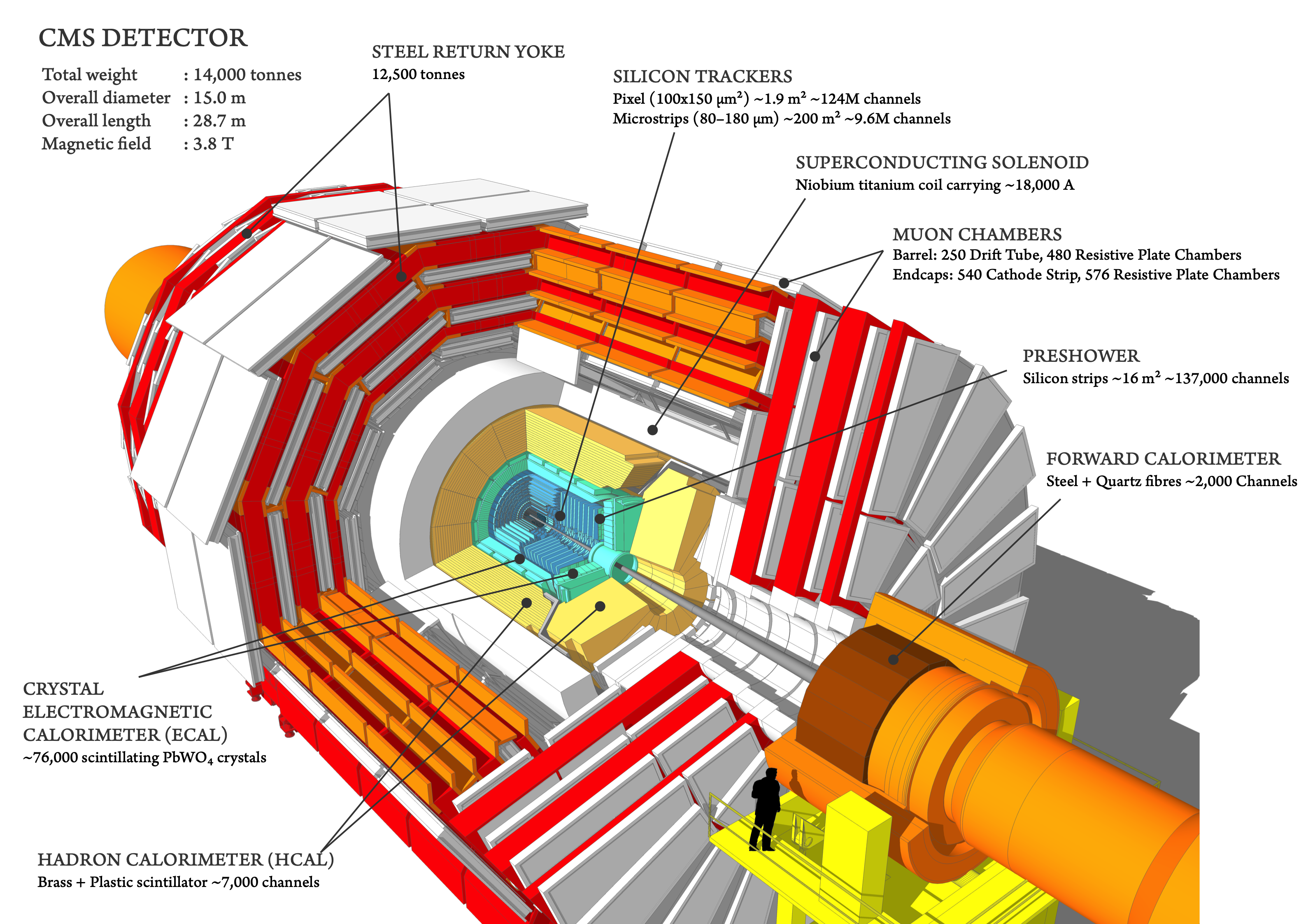
Of the several sophisticated detectors arrayed around the LHC ring, this thesis focuses on the Compact Muon Solenoid (CMS) detector. CMS is composed of several subdetector systems:
- Silicon trackers
- Crystal electromagnetic calorimeter (ECAL) and preshower detector
- Hadron calorimeter (HCAL)
- Superconducting solenoid magnet
- Muon chambers
[@Fig:cms_overview] shows how these subdetectors are assembled together, and each of these will be discussed in the following sections.
 {#fig:cms_overview}
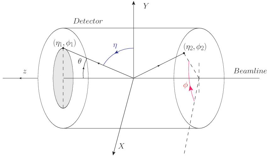
The CMS coordinate system ([@fig:cms_coordinate_system]) has its origin at the geometrical center of the detector. The Cartesian ordinals are:
- x-axis: pointing toward center of LHC ring
- y-axis: pointing vertically upward
- z-axis: pointing along the beam axis
A cylindrical coordinate system is also commonly used due to the overall cylindrical geometry of the detector. It uses the standard cylindrical definitions, $R=\sqrt{x^2+y^2}, \phi=\tan^{-1}\frac{y}{x}$.
 {#fig:cms_coordinate_system width=90%}
Other useful quantities in hadron colliders are the kinematic quantity known as rapidity, $y$, and a related geometrical quantity, pseudorapidity, $\eta$.
$$ y = \frac{1}{2}\mathrm{ln}\frac{E + p_z}{E-p_z} \quad \eta = -\mathrm{ln}\left( \frac{\theta}{2} \right) $$
Rapidity is a useful observable because it is Lorentz invariant for boosts along the beam axis, meaning that it is not dependent upon the particular rest frame of the two interacting partons in the event. However, rapidity is difficult to measure so the alternative, purely geometric quantity, pseudorapidity is used which approximates the rapidity as
$$ y \approx \eta - \frac{p_L}{2 |\mathbf{p}|} \left( \frac{m}{p_T} \right)^2 $$ In the ultra-relativistic limit $\left( \frac{m}{p_T} \rightarrow 0 \right)$ or for massless particles the approximation becomes exact.
Finally, the azimuthal angle, $\phi$, and the pseudorapidity are used to define the angular separation between particles as
$$ \Delta R = \sqrt{ \left(\Delta\phi\right)^2 + \left(\Delta\eta\right)^2 } $$
Silicon Tracking System
The silicon tracker consists of many layers of silicon pixel and strip detectors that record where charged particles pass through each individual layer. Sophisticated tracking software is then used to link together individual "hits" in the layers to form a coherent track describing the real path of the particle.
Both pixel and strip silicon detectors operate on the same principle. A sheet of silicon, typically a few hundred microns thick, is fabricated with a p-n junction running through it. Electrically it is little more than an diode. A typical diode used in electronics preferentially allows current to flow through it in one direction leading to a current vs voltage (IV) curve as shown on the left of [@fig:pixel_revbias]. As shown in the figure, a negative voltage above $V{\mathrm{br}}$ reverse biases the diode. In this state, all mobile charge carriers have been evacuated from the bulk. However, if the reverse voltage continues to grow, external charge carriers will be able to jump across the junction, leading to "breakdown" and a large increase in current. During manufacturing, silicon for particle detectors goes through qualification that ensures its breakdown voltage is high enough to operate efficiently. The right plot in [@fig:pixel_rev_bias] shows the current vs reverse voltage for several silicon detector sensors.
![]() {#fig:pixel_rev_bias}
{#fig:pixel_rev_bias}
When a silicon sensor is reverse-biased, there is normally only a tiny "leakage" current that flows through it. However, when an energetic charged particle such as an electron, muon, proton, etc. passes through the sensor, it interacts with the atoms in the material to raise orbital electrons into the conduction band of the semiconductor. This creates electron-hole pairs that drift apart due to the electric field resulting from the reverse bias voltage. Eventually, the electrons reach the surface where they are collected by conductive strips (strip detector) or bump bonds (pixel detectors) to be fed into a nearby readout chip. This is illustrated in [@fig:sensor_drift]
 {#fig:sensor_drift}
The original CMS tracker had three layers of pixel detectors in the barrel region (BPIX) and two on each forward region (FPIX) ([@fig:phase0_tracker]). In 2017, an upgraded version of the pixel detector, the Phase-I upgrade, was installed that increased the number of layers to four in the barrel and three in each forward region. For both detectors, the pixels were 100 $\mu \mathrm{m}$ by 150 $\mu \mathrm{m}$. More information on the upgrade project and the pixel detector can be found in chapter 6.
![]() {#fig:phase0_tracker}
{#fig:phase0_tracker}
Surrounding the pixel detector is the silicon strip tracker. As shown in [@fig:strip_tracker], the strip tracker has four sections: the inner (TIB) and outer (TOB) barrel, the inner disks (TID), and the endcap (TEC). The pitch of the strips in the different sections has been tuned to balance reconstruction precision, occupancy, and construction practicality, resulting in strips ranging in width from as small as 80 $\mu\textrm{m}$ in the TIB to 180 $\mu\textrm{m}$ in the outer layers of the TOB and TEC. The strips are oriented along the z-axis for the barrel and along the radial direction for the endcap layers. There are also two layers of double-sided strip detectors in the TOB with one side rotated 100 mrad relative to the other. Together, these two sides can give a 3D position measurement[@Fernandez2007].
![]() {#fig:strip_tracker}
{#fig:strip_tracker}
Electromagnetic Calorimeter
After leaving the tracker, particles reach the ECAL. Electrons and photons interact with the material in the crystals to create an electromagnetic shower. The shower occurs when electrons interact with the atoms of the material to radiate bremsstrahlung, or braking, photons. If the photons are energetic enough, they also interact with the material to produce electron-positron pairs which will continue the shower. This process continues until the particles no longer have enough energy to support the aforementioned processes. The deposition of energy from the shower into the ECAL crystals is used to help reconstruct photons and electrons in the original event.
The ECAL used by CMS is built with 75,848 lead tungstate ($\mathrm{PbWO}_4$) crystals. Lead tungstate was chosen for its high density (8.3 g/$\mathrm{cm}^3$), and short radiation length ($X_0$=0.89 cm). It it also desirable because it tends to produce well-collimated, narrow showers, having a Molière radius of 2.2 cm. The electromagnetic showers inside the ECAL crystals produce scintillation light which is captured and amplified by avalanche photodiodes (APDs).
To augment the ECAL, the preshower detector (ES) is installed just inside the forward ECAL. It addresses a peculiar issue resulting from neutral pions. These particles will commonly be produced with high enough momentum that when they decay ($\pi^0\rightarrow \gamma \gamma$), the photons will be so narrowly separated that the ECAL is at risk of identifying them as a single very high energy photon. Because Higgs searches were an important driver in the design of CMS, and $H\rightarrow \gamma \gamma$ was a potential discovery channel, the ES was added to help reduce the number of $\pi^0$ misidentified as high energy photons. The ES is constructed with alternating layers of lead and silicon detector, the first to initiate a shower and the second to give a high precision measurement of the shower-in-progress. This gives sufficient granularity to identify the narrowly separated photons from $\pi^0$ and other di-photon resonances.
 {#fig:ecal}
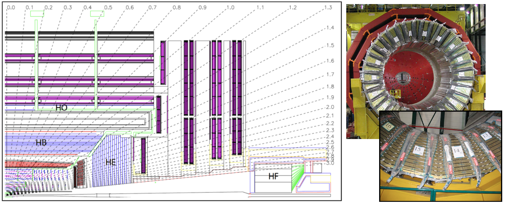
Hadron Calorimeter
Electrons and photons are effectively stopped in the ECAL. What remains are muons and hadrons. The muons continue largely unimpeded through the HCAL, but hadrons are stopped by the dense layers of brass and scintillating plastic. The HCAL operates on a similar principle to the ECAL, except the initial reaction is mediated by the strong force as an incident hadron interacts with an atomic nucleus of material in the HCAL. The products of this reaction may go on to have additional nuclear interactions, if they are themselves hadrons, or start electromagnetic showers if they are photons or electrons. The brass layers serve as the absorber, the material chosen for being non-ferromagnetic and having a short interaction length ($\lambda_I = 16.42$ cm). Scintillators equipped with silicon photomultipliers (SiPM) sample the hadronic "shower" as it traverses a particular layer. These samples are then used to calculate the energy of the initial particle.
The HCAL is divided into a barrel region (HB) and endcaps (HE) in the forward regions that sit inside the solenoid coil. There is also an additional layer (HO) that sits outside the magnet to provide a cumulative 11 interaction lengths of material so the shower is completely captured within the calorimeter. The HCAL regions are themselves sectioned in $\phi/\eta$ into towers.
 {#fig:hcal}
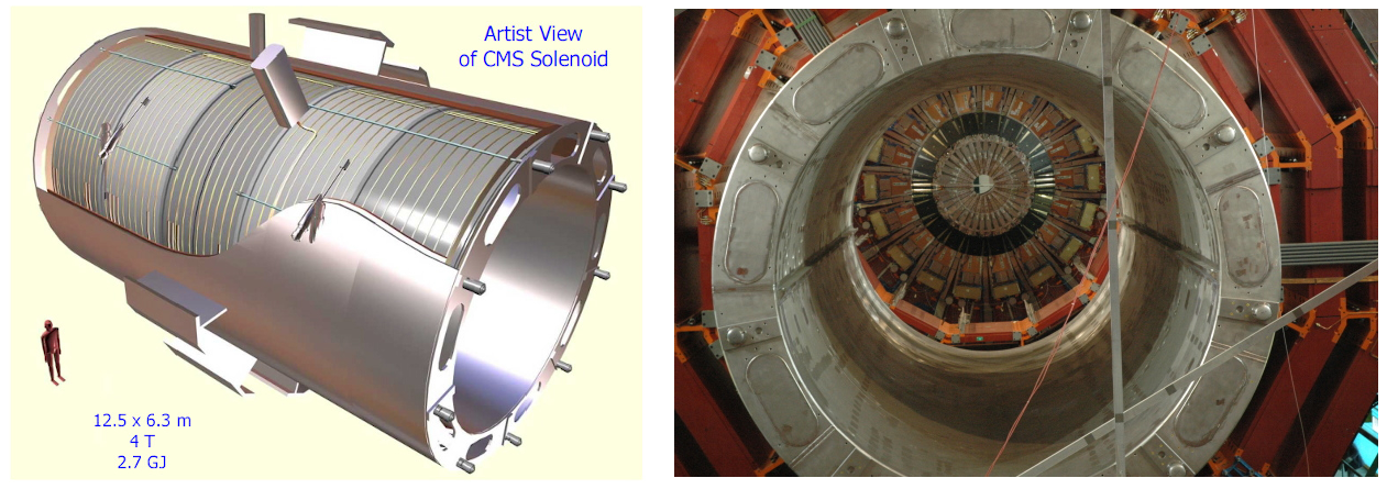
Superconducting Solenoid Magnet
A defining feature of the CMS experiment is its incorporation of a powerful superconducting solenoidal magnet ([@fig:cms_magnet]). It measures 6.4 m in diameter and weighs 12,000 tonnes. It can produce a very uniform 3.8 T magnetic field throughout the interior of the solenoid. The coil wire is made of a Ni-Tb alloy and must be cooled to 4.7 K with a helium cryogenic to achieve superconductivity. Under normal operating conditions, the cable carries over 18000 amps of current. Magnetic field lines run in loops, which means that there will be a return field on the outside of the solenoid. The shape of the return field is controlled through the iron return yoke, which is seen painted red in [@fig:cms_magnet;@fig:cms_overview].
 {#fig:cms_magnet}
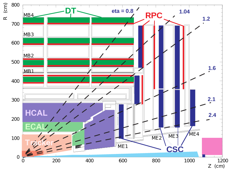
Muon System
Interleaved with the iron return yoke mentioned in the previous section, and putting the muon in Compact Muon Solenoid is the muon system. Besides neutrinos, which are not directly detected by CMS, muons are the only particle that normally escape the calorimeters and make it to the muon system. This makes identifying muons relatively trivial since any hits in the muon system must be from muons. Unlike the subsystems discussed so far, the muon system incorporates a diverse array of detector types into its design, as is shown in [@fig:muon_system]. The barrel section of the muon system uses drift tubes (DT), [@fig:drift_chambers], interspersed with resistive plate chambers (RPC). The forward region uses cathode strip chambers (CSC) with resistive plate chambers as well. The motivation for employing different types of detectors stems from the different conditions in the barrel vs forward region. In the forward region, there is a more intense residual magnetic field making drift tubes inappropriate, thus leading to the use of CSCs. The RPCs were used to add redundancy to the system for use as in the muon trigger.
 {#fig:muon_system}
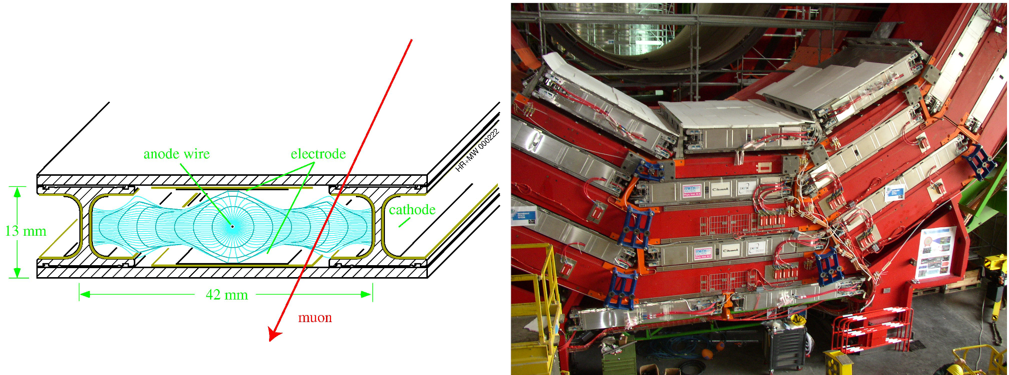 {#fig:drift_chambers}
The Trigger System and Data Handling
Every event recorded by CMS consists of roughly 1MB of data. With bunch crossings occurring every 25 ns, that corresponds to a veritable flood of data that would be technologically infeasible to handle (3.5 Exabytes per day!). To solve this problem, a sophisticated trigger system was developed to only select a small subset of events for further processing and analysis. The trigger system is divided into two parts: the Level 1 (L1) trigger which triggers a readout of the entire detector, and the High Level Trigger (HLT) that decides if a newly acquired event is saved to disk for offline analysis.
The L1 trigger provides a rate reduction of three orders of magnitude, down to a rate of roughly 100 kHz. It does this by processing information from just the calorimeters and muon system on custom hardware consisting of both FPGA and ASIC processing units. Some of these processing units are embedded within the detector and others are located in the nearby counting room. The schema for how this information is processed is shown in [@fig:l1_trigger]. The L1 trigger is designed to use information from just part of the detector to quickly (within 3.8 $\mu \mathrm{s}$) identify particles with high momentum transverse to the beam axis. It uses these high transverse momentum particles to decide whether to trigger a readout of the rest of the detector.
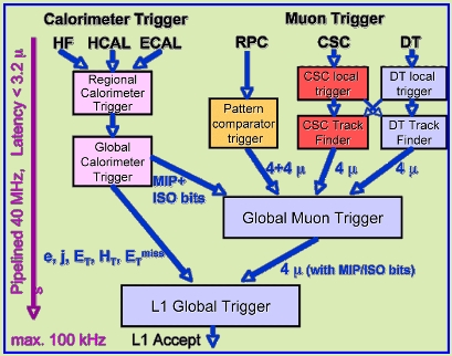 {#fig:l1_trigger width=60%}
If an event passes the L1 trigger, it is further scrutinized by the HLT. The HLT runs on a dedicated server farm that does an initial reconstruction of the event. There is a complex set of criteria that define many potential ways an event could pass the HLT. An example criteria could be a pair of electrons with very high momentum. Another could be a single very high energy muon. These different categories have been crafted to ensure that events having the signatures of interesting physics processes will be retained. To keep the total rate of events passing the HLT around 1000 Hz, some categories with naturally higher rates are prescaled, which means that a certain fraction of those events are discarded.
Events that pass the HLT are saved to disk, at which point the "Tier 0" computing cluster on the surface above the CMS cavern performs a full reconstruction. From that point, reconstructed events are collected into data sets based on which HLT paths they satisfied and when the events were collected. These data sets are then made available to the worldwide grid of computing resources for physicists to analyze.
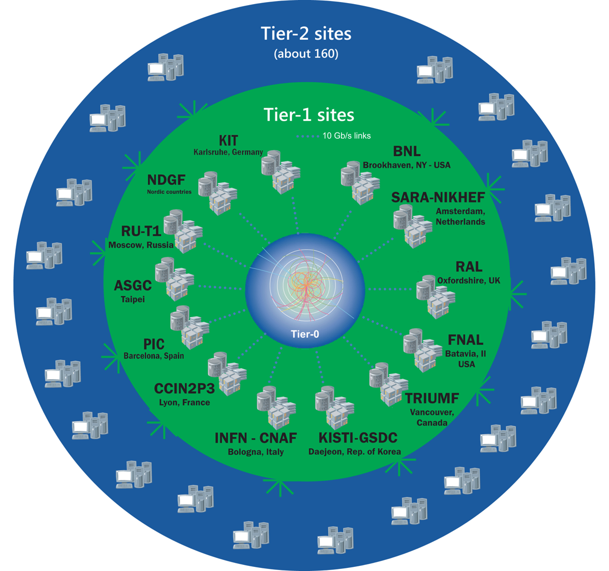
The Worldwide LHC Computing Grid (WLCG) is responsible for providing physicists and other users access to the data collected at LHC experiments and processing resources to analyze that data. The organization is organized into four tiers, shown in [@fig:cms_computing], each of which serves an important purpose.
- Tier 0: Physically split between two locations, CERN and the Wigner Institute computing center in Budapest, Hungary, the Tier 0 is responsible for the transformation of the raw data into a more compact form that can be distributed to the lower tiers, as well as providing quality control metrics that operators can use to monitor the accelerator and detector during operation.
- Tier 1: There are 13 Tier 1 sites. Normally hosted at large national computing centers, they are equipped with sufficient storage for LHC data sets and can handle large-scale reprocessing and safe-keeping of the corresponding output. They are also responsible for distributing data sets to Tier 2 facilities and storage of simulated data sets generated at Tier 2s.
- Tier 2: There are 160 Tier 2 facilities on the Grid. They are typically housed at universities and other scientific institutions. They can store sufficient data and provide adequate compute resources for user analysis tasks.
- Tier 3: These are the machines that individual analysts access to perform their analysis tasks. They are typically associated with a specific Tier 2 facility, but can provide access to Grid resources around the globe.
 {#fig:cms_computing}