thesis/content/02_standard_model.md

---

title: Brief Review of the Standard Model ...

The Standard Model of Particle Physics (SM) stands as one of the most predictive and insightful scientific theories ever written. It is the culmination of a hundred years of intense theoretical exploration and experimental tests. It can successfully explain phenomena ranging from nuclear decay and the structure of atoms to the behavior of cosmic ray showers. Included in the theory are three fundamental forces. The first and most familiar is the electromagnetic force which is mediated by the photon in which all particles with electric charge participate. The second is the strong nuclear force. The strong force is mediated by the gluon which controls the interaction between all particles possessing color charge. It is this force that is responsible for binding quarks together into mesons and baryons, as well as binding protons and neutrons together into atomic nuclei. Finally, the weak nuclear force, which is mediated by the W and Z bosons, and is responsible for nuclear $\beta$-decay as well as more exotic processes such as interactions with the ghostly neutrino particle and the decay of the heavy flavor quarks.

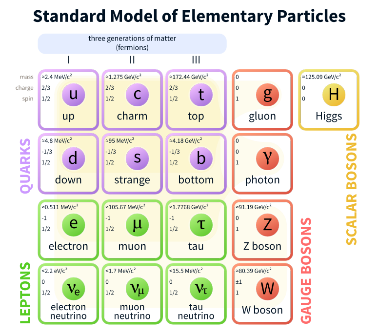
Notably, the Standard Model is completely unable to explain why apples fall from trees or why the earth orbits the sun since it does not incorporate the gravitational force. The current most complete theory of gravity is General Relativity. However, despite large and ongoing efforts to unite General Relativity with the Standard Model, no resulting theories have had the necessary self-consistency and predictive power to be accepted. Luckily for those working on collider experiments, the effect of gravity is so overwhelmed by the other three fundamental forces that it can be largely ignored. The constituent particles of the SM are shown in [@fig:sm_particles].

Fundamental Particles

The fermions are characterized by their half-integer spin of $\frac{1}{2}\hbar$ and are split between the leptons and the quarks. They are fundamentally defined as Dirac spinor fields, $\psi$, which in the case of non-interacting massive particles are described by the Lagrangian $$ \mathcal{L} = \bar{\psi}\left(i\partial!!!/ - m\right)\psi $$ {#eq:freefermion} in natural units, $\hbar=c=1$. The $\partial!!!/$ operator is defined as $\gamma^\mu\partial\mu$ in Einstein notation where $\gamma^\mu$ are the 4x4 $\gamma$-matrices that satisfy the anti-commutation relations $\left{\gamma^\mu,\gamma^\nu\right}=2\eta^{\mu\nu}$ and $\eta^{\mu\nu}$ is the Minkowski metric. Other fermions and interactions can be added to the theory with additional terms, as will be discussed in subsequent sections.

The leptons come in three generations with each generation having an electrically charged member and a neutral member. The charged members are the electron, muon, and tauon (or simply tau), while the neutral members are corresponding neutrinos. The electrically charged leptons participate in the electromagnetic and weak interactions, while the neutrinos only participate in the weak interaction. Another feature of the leptons is that while the charged leptons have non-trivial masses($me=511$ keV, $m\mu=106$ MeV, $m_\tau=1.78$ GeV), the neutrinos are nearly massless. In fact, they were originally believed to be massless, until the observation of neutrino-mixing implied that at least two of them must have mass. The quarks also come in three generations with two members in each generation. In contrast with the leptons, however, the quarks all carry electric charge. The "up-type" quarks carry charge $+2/3$ while the "down-type" quarks carry charge $-1/3$. The quarks are also colored which means that in addition to participating in the electromagnetic and weak interactions, they also interact via the strong nuclear force. Each of the six quarks has non-trivial mass, but they are wildly different, running from 2.4 $\mathrm{MeV}/\mathrm{c}^2$ for the up quark all the way to 171 $\mathrm{GeV}/\mathrm{c}^2$ for the top quark, the heaviest fundamental particle in the SM.

The remaining particles are the bosons: four force-mediators and the Higgs. These will be discussed in the following sections in context with their respective forces and contributions to the SM.

{#fig:sm_particles}

Quantum Electrodynamics

One of the early triumphs of quantum field theory (QFT) was the description of electromagnetism developed by Tomonaga[@Tomonaga1946], Schwinger[@Schwinger1948], Feynman[@Feynman1949], and Dyson[@Dyson1949] and eventually coming to be known as quantum electrodynamics (QED). This theory describes the interaction of electrically charged particles with photons. In QED photons are described by a 4-vector field, $A^\mu$, which is used to define the field strength tensor $F^{\mu\nu} = \partial^\mu A^\nu - \partial^\nu A^\mu$. This field, in the absence of charged particles, is governed by the Maxwell Lagrangian

$$ \mathcal{L}{\mathrm{Max}} = -\frac{1}{4}F^{\mu\nu}F{\mu\nu} $$

Interactions of the field with a fermion of charge $q$ can be added to [@eq:freefermion], which gives $$ \mathcal{L}{\mathrm{Int}} = \bar{\psi}\left(iD!!!!/ - m\right)\psi + \mathrm{h.c.} $$ where $D!!!!/ \equiv \gamma^{\mu}\left(\partial\mu + iqA\mu\right)$ and h.c. is just the hermitian conjugate of the previous term. Putting these together yields the QED Lagrangian: $$ \mathcal{L}{\mathrm{QED}} = i\bar{\psi}\gamma^\mu\partial\mu\psi - q\bar{\psi}\gamma^\mu A\mu\psi - \frac{1}{4}F^{\mu\nu}F{\mu\nu} - m_e \bar{\psi}\psi $$

QED is a gauge theory. This comes from the assumption that the observable is not the potential $A^\mu$, but only the physical fields it defines, which leads one to ask what transformations can be applied to $A^\mu$ that leave these fields invariant. The transformations that possess this feature are called gauge transformations, and these define symmetries of the theory. In the language of group theory, QED obeys $U(1)$ symmetry. The transformation associated with this symmetry that leaves $\mathcal{L}_{\mathrm{QED}}$ unchanged is: $$ A^\mu \rightarrow A^\mu + \partial^\mu \chi, \psi \rightarrow e^{-iq\chi}\psi $$ where $\chi$ is a constant for a global gauge symmetry, but varies arbitrarily over space-time for a local gauge symmetry. The symmetries in the SM are local gauge symmetries.

Enforcing a local gauge symmetry upon a Lagrangian severely limits the form of the terms that can appear. For example, a mass term for the photon field of the form $m\gamma A^\mu A\mu$ is forbidden. This is acceptable in QED since the photon is massless, but will prove to be an issue for the massive bosons that come with the weak force, as will be discussed shortly.

Feynman Diagrams and Cross Sections

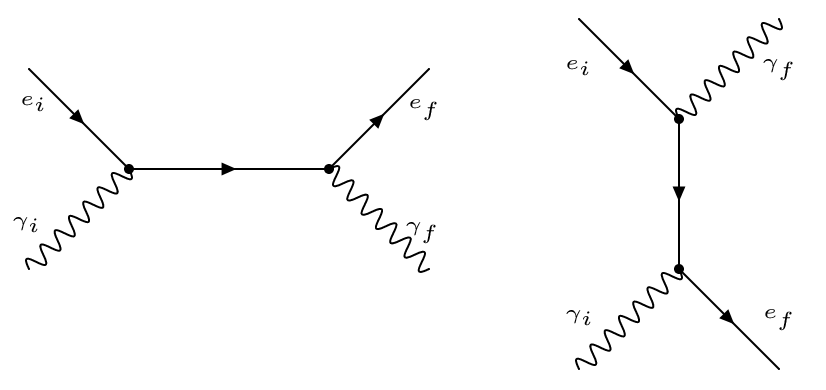
Observables in QFTs, especially in theories as complex as the SM, are rarely possible to calculate exactly using analytical methods. The solution to this issue is to look for approximate solutions of the field equations using small perturbations about the vacuum. This approach requires a small parameter to use in the perturbative expansion. For QED this is, in natural units, the positron charge $e=\sqrt{4\pi\alpha}\approx 0.3$. This perturbative expansion results in many terms, each of which can be represented graphically as a Feynman diagram. These are graphs that encode the interactions of particles in an intuitive way. A illustrative example is Compton scattering. In this process, a photon is incident on a charged fermion. Experimentally, this is normally an X-ray or gamma ray incident upon an electron in some atomic orbital. The electron absorbs the photon and then re-emits it with a smaller momentum (longer wavelength) than it started with. It is technically possible for the photon to be re-emitted with a larger momentum, but this is referred to as anti-Compton scattering. In any case, the process can be represented by the two diagrams in [@fig:compton_scattering]. There is a formalism for translating these diagrams into a precise calculation that can be performed analytically for simple cases, but often require the assistance of numerical methods. A description of the full formalism is beyond the scope of this discussion, but briefly:

• Each vertex in the graph contributes a factor proportional to the electromagnetic coupling constant, $\sqrt{4\pi\alpha}$.
• Photons and fermions contribute individual propagators that involve their momenta and, in the case of the fermions, their masses.
• Performing the calculation gives the amplitude of that diagram, which is a complex-valued function of the incoming and outgoing particles' momenta and spins. The next step is to add together the amplitudes of all of the diagrams under consideration, and then take the absolute square of the sum.
• The detectors used in collider experiments are typically not sensitive to spin and the beams, especially for hadron colliders, are not polarized, so an extra step involves averaging over the initial spin states and summing over the final spin states.

{#fig:compton_scattering}

The precise rules are derived from the Lagrangian describing the system using the tools of QFT. The result of this full calculation is the differential cross section. This can be interpreted as a probability distribution where, given some initial state particles, it can predict the momentum distributions of the final state particles. Integrating the differential cross section over all initial and final states gives the total cross section, or just cross section. The diagrams of [@fig:compton_scattering] are just the two leading order (LO) diagrams, meaning that of all possible diagrams, these have the smallest possible number of vertices. Since each vertex contributes additional factors of the coupling constant $g_e\equiv\sqrt{4\pi\alpha}$, diagrams with additional vertices give smaller and smaller individual contributions to the total cross section. However, the issue is complicated by the fact that the total number of diagrams at each order of $g_e$ increases, and the manner of interference between the diagrams is often not clear without doing the full calculation. This is why precise predictions require the explicit inclusion of more complicated diagrams. The set of diagrams that include the next fewest number of vertices are referred to as next-to-leading order (NLO), and beyond that are the next-to-next-to-leading order (NNLO) diagrams which are sometimes included for very precise calculations. The order to which calculations are performed is generally motivated by the related experimental precision. NLO calculations are most often satisfactory for collider based measurements.

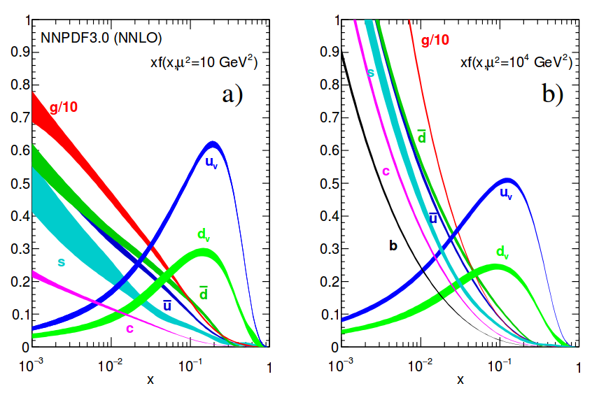
The cross section of any particular process depends upon the conditions facilitating that process. In hadron colliders, the (anti)protons that are collided are composite particles with three valence quarks as well as "sea" quarks and gluons that are continuously created and annihilated. When a high energy collision occurs, it is best understood as an interaction not between two protons, but of two of these constituent particles, or partons. Each of these partons carries a fraction of the proton's total energy, however this fraction is random and its probability distribution is different for each type of particle. These probability distributions are called the hadron's parton distribution functions (PDFs). [@Fig:proton_pdf] shows the PDFs for protons at different momentum transfer scales.

{#fig:proton_pdf}

Quantum Chromodynamics

The theory describing the interaction of particles with color charge is quantum chromodynamics (QCD). The colored fermions, quarks, were first proposed by Gell-Mann[@GellMann1964] and Zweig[@Zweig:1964jf] in 1964 to aid in the classification of hadrons, and were first observed four years later at SLAC[@Bloom1969]. In contrast with QED, QCD obeys the non-Abelian SU(3) symmetry, and just as $A^\mu$ was used to define a field strength tensor in QED, the eight gluon fields each define their field strength tensor as $$ G{\mu\nu}^{a} = \partial\mu G\nu^a - \partial\nu G_\mu^a - gs f{abc}G\mu^b G\nu^c $$ where $gs$ is the strong coupling constant and the $f{abc}$ are the structure constants of the symmetry group defined by the commutation relations $$ \left[\frac{\lambda_a}{2},\frac{\lambdab}{2}\right] = i f{abc} \frac{\lambda_c}{2} $$ where $\lambda_a$ are the Gell-Mann matrices. The quarks, similar to the fermions in QED, are represented as spinor fields governed by the Lagrangian $$ \mathcal{L}_q = \bar{qf}\left(i\gamma^{\mu}\partial\mu - m\right)q_f $$ for a single quark. In $\mathcal{L}_q$, $q_f = (\psi_1, \psi_2, \psi3)$ where each $\psi$ represents a color component and there is an implied sum over all three. Interactions between the quarks and the gluons are introduced by adding the covariant derivative $D\mu$ into $\mathcal{L}q$ in place of $\partial\mu$ where $$ D\mu = \partial\mu + ig_s\frac{\lambdaa}{2}G^a\mu. $$ Doing this yields the QCD Lagrangian. $$ \mathcal{L}_\mathrm{QCD} = \sum_f \bar{q}f\left(i\gamma^\mu\partial\mu - m\right)q_f - \frac{1}{4}Ga^{\mu\nu}G^a{mu\nu} - g_s \bar{q}_f \gamma^\mu \frac{\lambda_a}{2}qf G^1\mu $$ Coupling constants are generally only constant at a particular energy scale. Considering more or less energetic processes can affect the coupling constant. This effect is described by the interaction's beta function, $\beta\left( \alpha \right) = \partial \alpha / \partial \log\left( \mu \right)$ where $\mu$ is some energy scale. The beta function for QCD in the Standard Model is $$ \beta\left( \alpha_s \right) = -\frac{7\alpha_s^2}{2\pi} $$ where $\alpha_s \equiv g_s^2/4\pi$. The fact that the beta function is negative implies that the coupling decreases with energy scale, or equivalently, increases with larger length scales. This leads to the property of asymptotic freedom, which simply refers to the shrinking coupling as interaction length scales shorten. The coupling constant being small at high energies also means that one can successfully apply perturbation theory as one would in QED in that context. However, at low energies, such as those of most bound states, perturbative approaches fail and other approaches, such as Lattice QCD are applied instead. Quarks and gluons are also subject to color confinement, which means that any observable particle must be color neutral, and since individual quarks and gluons carry color charge they cannot be observed in isolation. Instead, this color neutrality is achieved through collections of these particles that together possess equal quantities of the three colors, conventionally called red, blue, and green. Such is the case for baryons, with three quarks carrying one of each color charge. Color neutrality can also be achieved via a quark-antiquark pair possessing the same color, e.g. a green quark and an green anti-quark together make up a colorless meson. Colorless combinations of more than three quarks are theoretically possible, but not normally encountered. Colorless pairings of gluons, or glueballs, are also possible in theory, but have not been observed experimentally.

A consequence of these properties is the hadronization and fragmentation of high energy quarks and gluons into jets. Fragmentation is the process by which an energetic quark or gluon, generally resulting from a hard collision, radiates a cascade of less energetic particles, and hadronization is the process where these particles become bound together into a jet of hadrons. However, this process does not occur for the top quark for reasons that will be explored in the next section.

The Electroweak Interaction

In 1934, Fermi proposed an explanation for nuclear beta decay, $n \rightarrow p e^- \bar{\nu_e}$[@Fermi1934]. The explanation involved a new interaction that would come to be identified as the weak nuclear force. This was initially proposed to be a direct interaction involving all incoming and outgoing particles sharing a single vertex. However, over the next few decades experiments at higher energies would show that this was just a low energy approximation. In reality this process is mediated by a new force mediator, the W boson. The W boson is one of the mediating bosons of the weak force, a new fundamental interaction with a peculiar feature, parity violation.

In 1956 Yang and Lee suggested that parity is not conserved in weak interactions, based on their examination of kaon decays[@Lee1956]. The next year, this was confirmed in studies of nuclear beta decays by Wu[@Wu1957]. Conservation of parity, roughly speaking, means that physical systems that are unchanged by a reflection about some plane will continue to remain unchanged by the reflection as the system evolves. This property holds for QED and QCD, but not for weak interactions.

{#fig:beta_decay width=50%}

Fundamentally, this follows from the fact that the weak force acts differently on particles of different chiralities. Chirality is a Lorentz invariant quantity that corresponds to eigenvalues of the operator $\gamma^5 = i\gamma^0\gamma^1\gamma^2\gamma^3$. Any field can be divided into chiral states with eigenvalues of +1, known as right-handed, and -1, known as left-handed. Chirality is related to the more familiar quantity of helicity. Helicity is the projection of a particle's spin along the direction of its momentum. Helicity, however, is not a Lorentz invariant quantity because a change of reference frame, or boost, can reverse the direction of the momentum, and with it the sign of the helicity. However, for massless particles one cannot reverse the momentum with a boost and the helicity and chirality are equivalent.

In the 1960's, work by Glashow[@Glashow1961], Salam, Ward[@Salam1964], and Weinberg[@Weinberg1967] showed that within the unified framework of their electroweak theory, a new spin-1 electrically charged particle should exist to mediate the weak force. This new particle, the W boson, was discovered at CERN in 1983 by the UA1[@Arnison1983a] and UA2[@Banner1983] experiments. Its mass is currently measured to be $MW=80.379\pm0.012$ GeV/$c^2$[@PhysRevD.98.030001]. The fields associated with the W boson, $W\mu^\pm$ couple only to the left components of fermion fields, implying that only left-handed particles and right-handed anti-particles can interact with the $W^\pm$ bosons. The symmetry group obeyed by this electroweak theory that generates these properties is $SU(2)_L\otimes U(1)_Y$.

The weak interaction does not directly couple to the fermions in their mass eigenstates, but rather superpositions of them. This mixing is described by the CKM (Cabibbo-Kobayashi-Maskawa) matrix for quarks and the PMNS (Pontecorvo-Maki-Nakagawa-Sakata) matrix for the leptons. The top quark, in particular, due to being heavier than the W boson, can decay weakly to an on-shell[^1] W boson and a bottom quark. This process happens on the timescale of $10^{-25}$ s which is smaller than the timescale necessary for top-flavored hadrons or $t\bar{t}$-quarkonium bound states to form[@Bigi1986]. In addition, because $|V{tb}| \gg |V{ts}|,|V_{td}|$ in the CKM matrix, the top quark will predominantly decay into a $W$ with a bottom quark, rather than with a strange or down quark.

The bottom quark will fragment and form a bottom-flavored hadron. Because the bottom quark's transition rate to lower mass quarks is relatively small, it will typically survive long enough to travel a few millimeters before decaying and forming a jet with its origin displaced relative to the primary interaction. The W will immediately decay into either a pair of quarks, resulting in two jets, or a charged lepton and a neutrino.

[^1]: A particle is allowed to exist virtually (as an interior line in a Feynman diagram) with a "mass" different from its normal mass. Such particles are said to be off-shell, while particles which are created at their normal mass are on-shell. All observable particles are on-shell.

The electroweak theory also predicts the existence of an electrically neutral spin-1 particle. This particle, called the Z boson, was also observed by the UA1[@Arnison1983b] and UA2[@Bagnaia1983] experiments at CERN, and its mass is currently measured to be $91.1876\pm 0.0021$[@PhysRevD.98.030001].

Electroweak symmetry breaking and the Higgs field

As mentioned previously, massive bosons are incompatible with local gauge invariance, which is clearly at odds with the observation of the W and Z bosons. A potential solution to this was proposed by Higgs[@Higgs1964], Brout, Englert[@Englert1964], and Guralnik, Hagen, and Kibble[@Guralnik1964] in 1964. Their solution was to employ the concept of spontaneous symmetry breaking.

The solution begins by introducing a doublet of complex scalar fields, known as the Higgs field.

$$ \phi = \begin{pmatrix} \phi^+ \ \phi^0 \end{pmatrix} = \begin{pmatrix} \frac{1}{\sqrt{2}}\left(\phi_1 + i\phi_2\right) \ \frac{1}{\sqrt{2}}\left(\phi_3 + i\phi_4\right) \end{pmatrix} $$

Here, the $\phi_i$'s are real scalar fields. The Lagrangian that governs the evolution of these fields is

$$ \mathcal{L\phi} = \left(D\mu \phi\right)^\dagger \left(D^\mu \phi\right) - V\left(\phi\right) $$ where the covariant derivative $D\mu$ is here defined as $$ D\mu = \partial_\mu + i gw W^i\mu \frac{\sigma_i}{2} + i gY B\mu \frac{Y}{2} $$ and the potential, $V\left(\phi\right)$ is $$ V\left(\phi\right) = \mu^2 \phi^\dagger \phi + \lambda |\phi|^2, \left(\mu^2 < 0, \lambda > 0 \right) $$ In the above equations, $B_\mu$, and $W_i$ are the original electroweak fields, from which the photon, W, and Z boson fields are composed, and $g_Y$ is the coupling constant associated with the weak hypercharge. The weak hypercharge is related to the electric charge, $q$, and the third component of the weak isospin via $Y = 2(q - I_z)$. The parameters $\mu$ and $\lambda$ are free parameters that characterize the Higgs field.

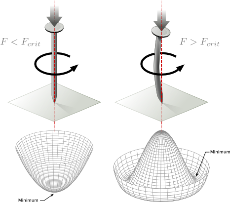
Critically, because $\mu^2 < 0$ the ground state is not at $\phi=0$, but instead has to satisfy $|\phi|^2 = -\frac{\mu^2}{2\lambda} \equiv \frac{v^2}{2}$. This is satisfied by an infinite number of ground states. Picking one breaks the $SU(2)_L\otimes U(1)Y$ symmetry obeyed by the original Lagrangian, $\mathcal{L}\phi$. [@Fig:symmetry_breaking] shows an analogue of this symmetry breaking in a familiar mechanical system. The particular ground state can be chosen freely, but a convenient choice is

$$ \phi_{gnd} = \begin{pmatrix} 0 \ \frac{v}{\sqrt{2}} \end{pmatrix} $$

{#fig:symmetry_breaking width=60%}

Combining $\mathcal{L}_\phi$ with the symmetry-broken electroweak Lagrangian and performing some simplification, we are left with:

\begin{align*} \mathcal{L} = &\frac{1}{2} \partial_\mu h \partial^\mu h - |\mu|^2 h^2 \

          -&\frac{1}{2} \left(W^-_{\mu\nu}\right)^\dagger W^{-\mu\nu} + \frac{1}{2}\left(\frac{g_w v}{2}\right)^2\left(W_\mu^-\right)^\dagger W^{-\mu} \\
          -&\frac{1}{4} \left(W^+_{\mu\nu}\right)^\dagger W^{+\mu\nu} + \frac{1}{2}\left(\frac{g_w v}{2}\right)^2\left(W^+\mu^-\right)^\dagger W^{+\mu} \\
          -&\frac{1}{4} Z_{\mu\nu}Z^{\mu\nu} + \frac{1}{2}\left(\frac{g_w v}{2\cos{\theta_W}}\right)^2 Z_\mu Z^\mu \\
          -&\frac{1}{4} A_{\mu\nu}A^{\mu\nu} \\
          +&\frac{g_w^2 v}{2} h W_\mu^- W^{+\mu} + \frac{g_w^2}{4}h^2 W_\mu^- W^{+\mu} + \frac{g_w^2 v}{4\cos^2{\theta_W}}h Z_\mu Z^\mu + \frac{g_w^2}{8\cos^2{\theta_W}}h^2 Z_\mu Z^\mu \\
          +&\frac{\mu^2}{v}h^3 + \frac{\mu^2}{4v^2}h^4

\end{align*}

In the above equation, $V{\mu\nu} \equiv \partial\mu V\nu - \partial\nu V_\mu$ for the W and Z vector bosons. This is best understood by looking through the terms line by line. The first line describes a spin-0 field, $h$, associated with a particle of mass $m_h = \sqrt{2}|\mu|$. This particle is the Higgs boson.

Lines 2-4 describe the spin-1 fields $W^\pm\mu$ and $Z\mu$. These fields are associated with the massive W and Z bosons that have been previously discussed. Their masses are related to fundamental constants as

$$ m_{W^\pm} = \frac{g_w v}{2} \quad \mathrm{and} \quad mZ = \frac{m{W^\pm}}{\cos\theta_W} $$

where $\theta_W$ is the Weinberg angle or weak mixing angle. It defines the spontaneous symmetry breaking angle that rotates the original neutral fields to obtain the Z boson and the photon. It is also relates the coupling strengths of the two electroweak sub-interactions

$$ e = g_w \sin\theta_W = g_Y\cos\theta_W $$

Line 5 describes the massless spin-1 field associated with the photon. Line 6 encapsulates the interaction between the vector bosons and the Higgs, and finally line 7 describes the Higgs self-interaction.

The Higgs mechanism itself only directly accounts for the masses of the vector bosons. While a significant victory, the masses of the fermions are still not included in the theory. This can be remedied by introducing Yukawa couplings between the fermions and the Higgs field. After spontaneous symmetry breaking, these contributions take the form

$$ \mathcal{L}_\mathrm{yukawa} = \sum -m_f \bar{\psi}\psi - \frac{m_f}{v}\bar{\psi}\psi h $$

The masses in the above equation are related to the Yukawa coupling which is unique for each particle and represents how strongly that particle interacts with the Higgs field. This relation is simply

$$ m_f = \frac{y_f}{2} v. $$

For most fermions, this coupling, $y_f$, is very small. For electrons it is roughly $2\times 10^{-6}$, for example. However, the top quark is unique in that its Yukawa coupling, $y_t$, is ~1 in the SM. This makes processes that involve interactions between the top quark and the Higgs boson interesting candidates for studying Higgs physics. In particular, the production cross section of four top quarks depends upon the value of the top Yukawa coupling. This is explored more deeply in chapter 5.