05_tttt_measurement.md 29 KB
title: Measurement of the $t\bar{t}t\bar{t}$ Cross Section at 13 TeV ...
Featuring high jet multiplicity and up to four energetic leptons, four top quark production is among the most spectacular SM processes that can occur at the LHC. It is also a rare process with a production cross section calculated to be $12.0^{+2.2}_{-2.5}\mathrm{fb}$ at Next-to-Leading Order (NLO) at 13 TeV center of mass energy[@Frederix2018]. Previous searches at ATLAS and CMS have set limits on the cross section of XXX[@TODO] and YYY[@TODO]. The goal of this analysis is to improve upon previous results by analyzing a larger dataset and utilizing improved analysis methods.
The production of four top quarks is possible through a variety of SM diagrams. [@fig:ft_prod_feyn] shows a few of these diagrams. The purely gluon mediated diagrams contribute roughly 90% of the total cross section, with electroweak and Higgs mediated diagrams contributing the remainder.
As discussed in chapter 2, top quarks are unique among quarks in that they are heavy enough to decay weakly. This results in them having the extremely short lifetime of around $5\times10^{-25}$s. This is much shorter than the timescale for hadronization (XXX) so they decay almost exclusively to a W boson and a bottom quark. Therefore, the final state particles of an event with top quarks are determined by the decay mode of the child W boson. Approximately 67% of W bosons decay to lighter flavor (ie not top) quark anti-quark pairs, while the rest will decay to $e$, $\mu$, and $\tau$ leptons in approximately equal probability. Electrons and muons can be observed directly while tauons will themselves decay to either $e/\mu$, or hadrons.
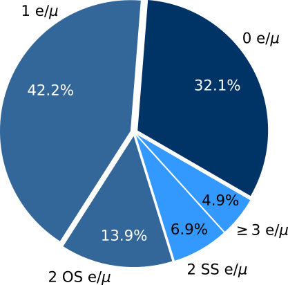
For four top quarks, the final states are conventionally defined in terms of the number and relative charges of $e/\mu$ leptons. This is summarized in [@fig:ft_final_states] with the coloring indicating the three analysis categories: fully hadronic, single lepton or opposite sign dilepton, and same-sign dilepton or 3 or more leptons, where lepton here and henceforth should be taken to mean $e/\mu$ unless otherwise noted.
Four top searches for each of these final state categories demand unique analysis strategies due to different event content and vastly different SM backgrounds. In particular, the same-sign dilepton and three or more lepton category benefit from a relatively small set of SM backgrounds at the expense of a rather small overall branching ratio. This is the category that is examined in this analysis[^1].
[^1]: The analysis description in this document omits some details for the sake of clarity. However, the analysis documentation[@CMSFT2019] contains all the technical details.
The basic strategy of this analysis is to first craft a selection of events that are enriched in $t\bar{t}t\bar{t}$. This is done by cutting on relatively simple event quantities such as the number and relative sign of leptons, number of jets, number of b-tagged jets, overall hadronic activity, and missing transverse momentum. A multivariate classifier is trained on simulated events within this selection to distinguish $t\bar{t}t\bar{t}$ from background events. This MVA produces a discriminant value that tends towards one for $t\bar{t}t\bar{t}$ like events, and to zero for background like events. This discriminant is then calculated for real and simulated events and divided into several bins. Finally, a maximum likelihood fit is performed on the discriminant distribution to extract the deviation of the measured distribution from the background-only distribution. A statistically significant (and positive) deviation can then be interpreted as evidence of $t\bar{t}t\bar{t}$ production.
Datasets and Simulation
This analysis uses data collected during 2016, 2017, and 2018 with the CMS detector. This corresponds to a total integrated luminosity of 137.2 fb$^{-1}$. Events that pass the HLT are divided into roughly disjoint datasets. Of the many of these produced by CMS, this analysis uses:
- DoubleEG/EGamma: two-electron channel
- DoubleMuon: two-muon channel
- MuonEG: crossed channel targeting events with one muon and one electron
- JetHT: used to recover efficiency for dilepton+$H_T$ triggers in period 2016H (although no additional events are found in this sample).
Because the datasets are not completely disjoint, care has been taken to avoid double counting events that may occur in multiple datasets.
Monte Carlo simulation is used extensively to model background and signal processes relevant to this analysis. See chapter 4 for more details on the process of producing simulated events. Samples of simulated Standard Model process events are produced centrally by a dedicated group within the CMS collaboration [@TODO]. Because detector conditions were changed year-to-year over Run 2, this analysis uses three sets of samples, one for each year. Each year's set of samples are then re-weighted to match the integrated luminosity of that year.
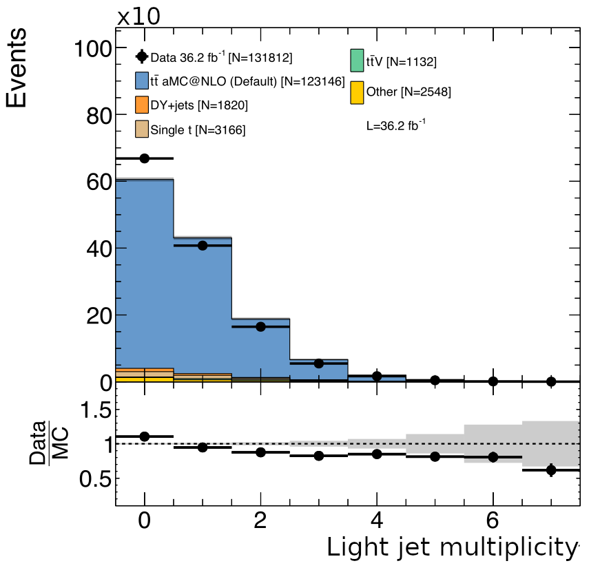
Because $N_{jet}$ is expected to be an important discriminating variable for $t\bar{t}t\bar{t}$, it is important to ensure that the spectrum of jets originating from initial state and final state radiation (ISR/FSR) is accurately modeled. This is particularly true for the major backgrounds $t\bar{t}W$ and $t\bar{t}Z$. The key observation to performing this correction is that a mismodeling of the ISR/FSR spectra by the event generator will be very similar between $t\bar{t}+X$ and just $t\bar{t}$. So by measuring the disparity between data and MC in $t\bar{t}$, correction weights can be obtained and applied to $t\bar{t}+X$. The number of ISR/FSR jets in data is obtained by selecting dilepton $t\bar{t}$ events with exactly two identified b-jets. Any other jets are assumed to be from ISR/FSR. The weights are then computed as the bin-by-bin ratio of the number of measured events with a certain number of ISR/FSR jets to the number of predicted events with that number of ISR/FSR jets. The results of this measurement for 2016 data and MC are shown in [@fig:isrfsr_correction].
The number of b-tagged jets is also expected to be an important discriminator for $t\bar{t}t\bar{t}$. Therefore, the flavor composition of additional jets in simulation should also be matched to data. Specifically, there has been an observed difference between data and simulation in the measurement of the $t\bar{t}b\bar{b}/t\bar{t}jj$ cross-section ratio[@CMSttbb]. To account for this, simulation is corrected to data by applying a scale factor of 1.7 to simulated events with bottom quark pairs originating from ISR/FSR gluons.
Object Definitions
This section describes the basic event constituents, or objects, that are considered in this analysis. The choice of the type and quality of these objects is motivated by the final state content of $t\bar{t}t\bar{t}$ events. These are electrons, muons, jets, b-tagged jets, and an imbalance of transverse momentum indicating the presence of neutrinos. Each of these objects has dedicated groups within the CMS collaboration that are responsible for developing accurate reconstruction and identification schemes for them. These Physics Object Groups (POGs) make identification criteria, or IDs, available for general use in the collaboration. Many analyses, including this one, incorporate these POG IDs into their own particular object definition and selection.
Electrons
Electrons are generally seen in two parts of the CMS detector: the tracker, and the electromagnetic calorimeter. One step in event reconstruction is to match tracks from the tracker with energy deposits in the ECAL. These electron candidates are then evaluated in one of a variety of schemes to determine the probability that it is from a genuine electron vs a photon, a charged hadron, or simply just an accidental match of two unrelated constituents. For this analysis, only electrons with $|\eta|<2.5$, i.e. within both the tracker and ECAL acceptance, are considered.
The particular scheme to determine the quality of an electron candidate employed for this analysis uses a multivariate discriminant built with shower-shape variables ($\sigma{i\eta i\eta}$, $\sigma{i\phi i \phi}$, cluster circularity, widths along $\eta$ and $\phi$, $R9$, H/E, $E{\mathrm{in-ES}}/E{\mathrm{raw}}$), track-cluster matching variables ($E{\mathrm{tot}}/p{\mathrm{in}}$, $E{\mathrm{ele}}/p{\mathrm{out}}$, $\Delta \eta{\mathrm{in}}$, $\Delta \eta_{\mathrm{out}}$, $\Delta \phi{\mathrm{in}}$, $1/E-1/P$), and track quality variables ($\chi^2$ of the KF and GSF tracks, the number of hits used by the KF/GSF filters, fbrem). Additional details on the construction and calibration of this discriminant can be found in [@TODO].
Charge mismeasurement of leptons can result in an opposite-sign dilepton event appearing as a same-sign dilepton event. Because there are potentially large backgrounds with opposite-sign dileptons, extra steps are taken to remove events with likely charge mismeasurement. In CMS, there are three techniques for measuring electron charge [@AN-14-164]. For the highest quality, or "tight", category of electrons used in the analysis, all three methods are required to agree. Electrons can also originate from photon conversion into electron-positron pairs. These photons will sometimes pass through one or more layers of the tracker before decaying, resulting in "missing" inner layer hits for the tracks of the child particles. Tight electrons are therefore required to have exactly zero missing inner hits. Consistency with having originated from the correct p-p interaction is also considered by applying cuts on the impact parameter, or the vector offset between the primary vertex and the track's point of closest approach to it. In particular, there are cuts on $d_0$, the transverse component of the offset, $dz$, the longitudinal component, and $SIP\mathrm{3D}$, the length of the offset divided by the uncertainty of the vertex's position.
Muons
Muons are reconstructed in CMS by matching energy deposits in the muon system to tracks in the tracker. The individual quality of the tracker and muon system contributions as well as the consistency between them are used to define IDs. The muon POG defines two IDs that are used in this analysis: loose[@MuId], and medium[@muonMediumId]. Only muons within the muon system acceptance $|\eta|<2.4$ are considered, and the same impact parameter requirements are applied as for electrons. For muons, the length and double-bend of the track implies that charge mismeasurement is small, however a requirement on the track quality is still applied $\delta p_T(\mu) / p_T(\mu) < 0.2$.
Lepton Isolation
The uniquely crowded environment of $t\bar{t}t\bar{t}$ and its main background prompted the development of a specialized isolation requirement, known as multi-isolation[@AN-15-031]. It is composed of three different variables
The first component is mini-isolation. A requirement on $I_\mathrm{mini}$ ensures that lepton is isolated, properly adapting to boosted topologies. It does this by having a variable sized cone that becomes tighter as the lepton's energy grows. The size of this cone, $R\equiv \sqrt{\left(\Delta\phi\right)^2 + \left(\Delta\eta\right)^2}$, is defined by
$$ R = \frac{10}{\mathrm{min}\left(\mathrm{max}\left(p_T(\ell), 50\right), 200 \right)} $$
With this, $I_\mathrm{mini}$ is
$$ I_\mathrm{mini} = \frac{\sum_R p_T\left(h^\pm\right) - \mathrm{max}\left(0, \sum_R p_T \left(h^0\right) + p_T\left(\gamma\right) - \rho \mathcal{A}\left(\frac{R}{0.3}\right)^2\right)}{p_T\left(\ell\right)} $$
where the sums are over the transverse energies of the charged hadrons, neutral hadrons, and photons within the cone, and $\rho$ is the pileup energy density. The effective areas, $\mathcal{A}$, used in this analysis are shown in {@tbl:eff_area2016} and {@tbl:eff_area2017_2018}.
| $\mu$ - $|\eta|$ range | $\mu$ - $\mathcal{A}(\mu)$ neutral | $e$ - $|\eta|$ range | $e$ - $\mathcal{A}(e)$ neutral | | :--------------------: | :-------------------------------: | :------------------: | :----------------------------: | | 0.0 - 0.8 | 0.0735 | 0.0 - 1.0 | 0.1752 | | 0.8 - 1.3 | 0.0619 | 1.0 - 1.479 | 0.1862 | | 1.3 - 2.0 | 0.0465 | 1.479 - 2.0 | 0.1411 | | 2.0 - 2.2 | 0.0433 | 2.0 - 2.2 | 0.1534 | | 2.2 - 2.5 | 0.0577 | 2.2 - 2.3 | 0.1903 | | | | 2.3 - 2.4 | 0.2243 | | | | 2.4 - 2.5 | 0.2687 |
: Effective areas used in 2016 {#tbl:eff_area2016}
| $\mu$ - $|\eta|$ range | $\mu$ - $\mathcal{A}(\mu)$ neutral | $e$ - $|\eta|$ range | $e$ - $\mathcal{A}(e)$ neutral | | :--------------------: | :-------------------------------: | :------------------: | :----------------------------: | | 0.0 - 0.8 | 0.0566 | 0.0 - 1.0 | 0.1440 | | 0.8 - 1.3 | 0.0562 | 1.0 - 1.479 | 0.1562 | | 1.3 - 2.0 | 0.0363 | 1.479 - 2.0 | 0.1032 | | 2.0 - 2.2 | 0.0119 | 2.0 - 2.2 | 0.0859 | | 2.2 - 2.5 | 0.0064 | 2.2 - 2.3 | 0.1116 | | | | 2.3 - 2.4 | 0.1321 | | | | 2.4 - 2.5 | 0.1654 |
: Effective areas used in 2017 and 2018 {#tbl:eff_area2017_2018}
The second variable used in the multi-isolation is ratio of the lepton $p_T$ to the $p_T$ of a jet matched to the lepton.
$$ p_T^\mathrm{ratio} = \frac{p_T\left(\ell\right)}{p_T\left(\mathrm{jet}\right)} $$
The matched jet is almost always the jet the contains the lepton, but if no such jet exists, the jet closest in $\Delta R$ to the lepton is chosen. The use of $p_T^\mathrm{ratio}$ is a simple approach to identifying leptons in very boosted topologies while not requiring any jet reclustering.
The third and final variable is the relative $p_T$. This is the the magnitude component of the matched jet's momentum transverse to the lepton's momentum divided by the difference between the jet and lepton momentum.
$$ p_T^\mathrm{rel} = \frac{|\left(\vec{p}(jet) - \vec{p}(\ell)\right) \times \vec{p}(\ell)|}{|\vec{p}(jet) - \vec{p}(\ell)|} $$
This helps recover leptons that are accidentally overlapping with unrelated jets.
These three variables are combined to create the multi-isolation requirement:
$$ I_\mathrm{mini} < I_1 \land \left( p_T^\mathrm{ratio} > I_2 \lor p_T^\mathrm{rel} > I_3 \right) $$
The three selection requirements, $I_1$, $I_2$, and $I_3$, are tuned individually for electrons and muons, since the probability of misidentifying a jet as a lepton is higher for electrons than muons.
These qualities are used to define three categrories of each flavor of lepton, tight, fakable, and loose. The selections for each of these categories is detailed in [@tbl:lep_selection].
| $\mu$-loose | $\mu$-fakable | $\mu$-tight | $e$-loose | $e$-fakable | $e$-tight | |
|---|---|---|---|---|---|---|
| Identification | loose ID | medium ID | medium ID | loose WP | loose WP | tight WP |
| Isolation | loose WP | loose WP | $\mu$ WP | loose WP | loose WP | $e$ WP |
| $d_0$ (cm) | 0.05 | 0.05 | 0.05 | 0.05 | 0.05 | 0.05 |
| $d_z$ (cm) | 0.1 | 0.1 | 0.1 | 0.1 | 0.1 | 0.1 |
| $SIP_\mathrm{3D}$ (cm) | - | $<4$ | $<4$ | - | $<4$ | $<4$ |
| missing inner hits | - | - | - | $\le 1$ | $=0$ | $=0 |
| tight charge | - | yes | yes | - | yes | yes |
: Summary of lepton selection {#tbl:lep_selection}
Jets
Jets are reconstructed from particle flow candidates that were clustered with the anti-kt alorithm with a cone size of $\Delta R < 0.4$. To be considered, jets must possess a transverse momentum $p_T > 40$ GeV and be within the tracker acceptance $|\eta| < 2.4$. To further suppress noise and mis-measured jets, additional criteria are enforced. For the 2016 data, jets are required to have
- neutral hadronic energy fraction < 0.99
- neutral electromagnetic energy fraction < 0.99
- number of constituents > 1
- charged hadron fraction > 0
- charged particle multiplicity > 0
- charged EM fraction < 0.99
For 2017 and 2018, an adjusted set of requirements were applied following the JetMet POG's recommendations. These are
- neutral hadronic energy fraction < 0.9
- neutral electromagnetic energy fraction < 0.9
- number of constituents > 1
- charged hadron fraction > 0
- charged multiplicity > 0
To avoid double counting due to jets matched geometrically with a lepton, the jet closest to a fakable or tight lepton with $\Delta R < 0.4$ is excluded from consideration as a jet in the event. From all jets that pass the stated criteria, a critical variable is calculated that will be used extensively in the analysis, $HT \equiv \sum\mathrm{jets} p_T$.
B-Jets
Hadrons containing bottom quarks are unique in that they typically have a lifetime long enough to travel some macroscopic distance before decaying, but still much shorter than most light-flavor hadrons. This leads to bottom quarks producing a jets not at the primary vertex but at a displaced vertex. This displaced vertex will typically be a few millimeters displaced from the primary vertex. One of the critical roles of the pixel detector is to enable such precise track reconstruction that the identification of these displaced vertices can be done reliably. This identification of b-jets is done by feeding details of the secondary vertex, and jet kinematics into a machine learning algorithm that distills all the information to a single discriminant. Different working points (WPs) are established along the discriminant's domain to provide reference performance metrics. Generally, a loose, medium, and tight WPs are defined which correspond to 10%, 1%, and .1% probabilities, respectively, to mis-tag jets from light quarks as bottom quark jets.
In this analysis, jets the pass all the criteria of the previous section, with the exception that the $p_T$ threshold has been lowered to 25 GeV, can be promoted to b-jets. The deepCSV discriminator is used in this analysis at the medium working point[@BTagging].
The jet multiplicity, $N_\mathrm{jets}$, and $H_T$ both include b-jets along with standard jets, provided that they have $p_T>40GeV$.
Missing Transverse Energy
When neutrinos are produced at CMS, they escape the detector while leaving no signals in any of the subdetectors. However, the presence of neutrinos can be inferred by an imbalance in the total transverse momentum of particles in an event. This observation comes from conservation of momentum where the partons in the initial interaction each have negligible momentum transverse to their beam directions which means that the sum of the transverse momenta of the final state particles must also be very small. By taking this sum over all visible particles, one can infer that any difference from zero must be from an invisible particle, or particles, which in the SM are neutrinos.
Event Selection
Before defining the baseline selection of events, it is good to review what the $t\bar{t}t\bar{t}$ signature is in the same-sign lepton channel.
- 2 same-sign leptons, including any combination of electrons and muons.
- 2 neutrinos associated with the aforementioned leptons through their parent W bosons
- 4 b-jets, one from each top quark
- 4 jets from two hadronic W decays
This analysis is also inclusive of the three and four lepton case. These are similar to the above except there are incrementally more leptons and neutrinos and fewer jets, although the number of b-jets remains constant. With that in mind, the baseline selection is the following:
- a pair of same-sign leptons satisfying the tight ID requirements.
- $N_\mathrm{jets} \ge 2$
- $N_\mathrm{b jets} \ge 2$
- $E!!/_T > 50$ GeV
- $H_T > 300$ GeV
- $p{T,\mathrm{lep1}} \ge 25 \mathrm{GeV}, p{T,\mathrm{lep2}} \ge 20 \mathrm{GeV}$
Events that contain a third lepton passing the loose ID that makes a Z-boson candidate (opposite-sign, same flavor pair with $|m_{\ell\ell} - mZ| < 12 \mathrm{GeV}$ or $m{\ell\ell} < 12 \mathrm{GeV}$) with one of the two same-sign leptons are rejected. However, if the third lepton passes the tight ID requirements and creates a Z-boson candidate and has a transverse momentum larger than 5 GeV for muons or 7 GeV for electrons, then the event is instead placed into a dedicated $t\bar{t} Z$ control region called CRZ.
If additional tight leptons do not form a Z candidate and have transverse momentum of at least 20 GeV, then they contribute to the lepton count for the event, $N_\mathrm{lep}$.
Events that pass the baseline selection and do not get discarded or placed into CRZ are divided into several signal regions. There are two approaches used in this analysis for defining these signal regions.
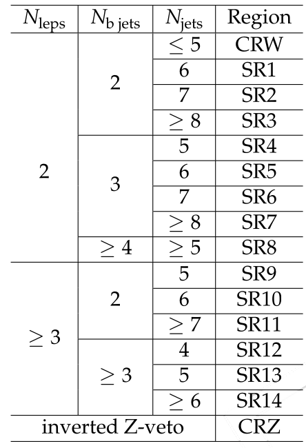
The first approach, called cut-based, is to categorize the events based on the number of leptons, jets, and b-jets. These regions are described in [@fig:cut_based_sr]. In the cut-based analysis, an additional control region was employed to help constrain $t\bar{t}W$ called CRW.
The other approach for defining the signal regions is to use a multivariate analysis (MVA) tool. In this analysis, a boosted decision tree (BDT) was used. This BDT used an expanded set of event information, relative to the cut-based classification, to construct a discriminator that would separate signal, i.e. $t\bar{t}t\bar{t}$, events from background events. This continuous discriminator value is then divided into several bins which will each contain events that have a discriminator value with the bounds of that bin.
Before the BDT can be used, it must be trained. Because BDT training is susceptible to overtraining unless a large number of training events are available. To avoid this issue, a relaxed baseline selection was created. It is
- Lepton 1 $p_T > 15$ GeV
- Lepton 2 $p_T > 15$ GeV
- $H_T > 250$ GeV
- $E!!/_T > 30$ GeV
- $N_\mathrm{jets} \ge 2$ GeV
- $N_\mathrm{b jets} \ge 1$ GeV
Signal was defined to be from $t\bar{t}t\bar{t}$ MC samples and background was taken to be all of the SM background processes described in the next section. Over 40 event-level variables were considered for the BDT inputs. Ranked in approximately descending order of discriminating power, as reported by the training routine of TMVA[], they are
- $N_\mathrm{jets}$
- $N_\mathrm{b jets}$
- $N_\mathrm{leps}$
- $M_T(\ell_2)$
- $m_{\ell_1\ell_2}$
- $E!!/_T$
- $M_T(\ell_1)$
- $H_T^b$: $H_T$ constructed from b-jets only
- $m_{j_1 j_2}$: invarient mass of two leading, i.e. highest $p_T$, jets
- $m_{l_1 j_2}$
- $\Delta\phi_{j_1 j_2}$
- $\Delta\phi_{\ell_1 j_1}$
- $p_T(j_i)$: $i \in [1,8]$
- $q_1$: sign of the same-sign lepton pair
- $\Delta \eta_{\ell_1 \ell_2}$
- $H_T$
- $H_T^\mathrm{ratio}$: Ratio of $H_T$ of first four leading jets to rest
- $m_{\ell_1 j_1}$
- $N_b^\mathrm{loose}$: Number of b jets passing the loose threshold
- $N_b^\mathrm{tight}$: Number of b jets passing the tight threshold
- $\mathrm{max}\left(m(j)/p_t(j)\right)$: highest ratio of jet mass to momentum to discriminate merged jets
- $N_\mathrm{w-cands}$: Number of jet pairs with invarient mass withing 30 GeV of the W mass
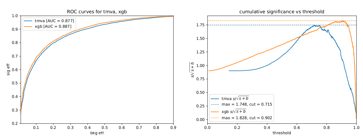
Other variables such as additional invarient mass pairings and angular information were considered but showed little to no discrimination power. This ranking takes into account the correlation between variables. This explains why, for example, $HT$ is ranked quite low. This is simply due to it being largely correlated with $N\mathrm{jets}$ and adding little additional information. In other words, this ordering can change significantly if certain variables are added or removed. Past approximately 22 variables, no extra discriminating power is gained in the BDT. This discriminating power is quantified by examining the Receiver Operating Characteristic (ROC) curve. The ROC curve is formed by calculating the signal efficiency and background rejection for different cuts on the discriminator value. Different working points can exist along this curve, but the discriminator overall performance can be quantified by calculating the area under the ROC curve (AUC). Of the variables listed above, 19 were chosen to continue optimization.
- $N_\mathrm{b jets}$
- $N_\mathrm{jets}$
- $N_b^\mathrm{loose}$
- $E!!/_T$
- $N_b^\mathrm{tight}$: Number of b jets passing the tight threshold
- $p_T(\ell_2)$
- $m_{l_1 j_1}$
- $p_T(j_1)$
- $p_T(j_7)$
- $\Delta\phi_{l_1 l_2}$
- $p_T(j_6)$
- $\mathrm{max}\left(m(j)/p_t(j)\right)$
- $N_\mathrm{leps}$
- $p_T(\ell_1)$
- $\Delta \eta_{\ell_1 \ell_2}$
- $p_T(j_8)$
- $H_T^b$
- $p_T(\ell_3)$
- $q_1$
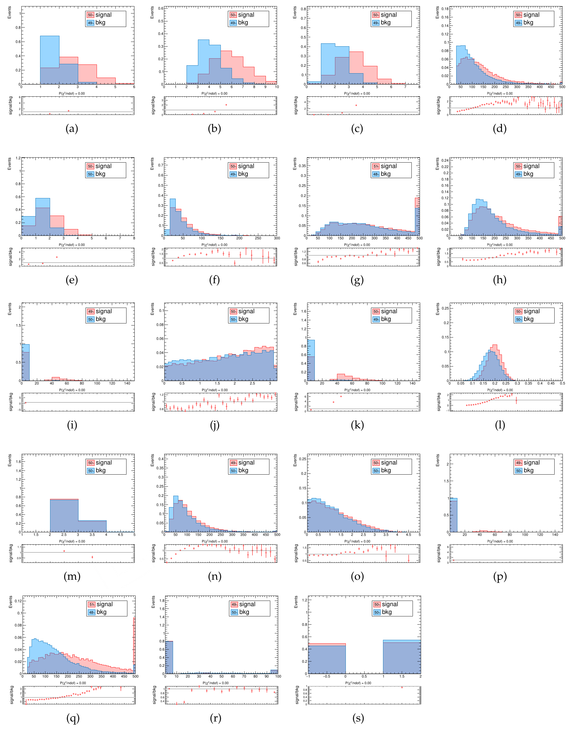
The kinematic distributions of these input variables are shown in [@fig:bdt_kinem].
In addition to the input variables, a BDT is described by several parameters internal to the algorithm. These parameters are referred to as hyperparameters. These change across different MVA algorithms and even between different implementations. In the case of BDTs in TMVA, the following hyperparameters were chosen and are listed with their optimized values.
- NTrees=500
- nEventsMin=150
- MaxDepth=5
- BoostType=AdaBoost
- AdaBoostBeta=0.25
- SeparationType=GiniIndex
- nCuts=20
- PruneMethod=NoPruning
An alternative library called xgboost was tested for comparison. Optimization of its BDT implementation resulted in the following hyperparameters. Note how set of hyperparameters is different from TMVA.
- n_estimators=500
- eta=0.07
- max_depth=5
- subsample=0.6
- alpha=8.0
- gamma=2.0
- lambda=1.0
- min_child_weight=1.0
- colsample_bytree=1.0
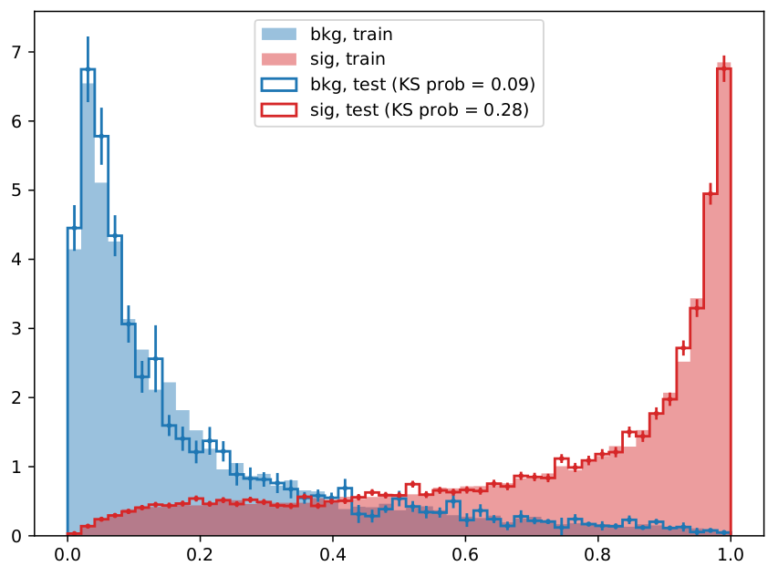
When comparing the above sets of hyperparameters, note that "n_estimators" is equivalent to "NTrees". "eta" is the learning rate for the xgboost BDT implementation. [@Fig:bdt_performance] shows a comparison between these two optimized BDTs, and [@fig:xgboost_disc_shape] demonstrates the signal separation achieved by the BDT.
The analysis that incorporates the BDT discriminant into the signal region definitions is here referred to as the BDT-based analysis. The BDT-based signal regions contain all of the same events as the cut-based signal regions. However, they are distributed into 17 bins based upon the events discriminant value and 1 bin for events in CRZ, giving 18 bins in total. Note that in contrast with the cut-based signal regions, there is no CRW control region in the BDT analysis. In this case, $t\bar{t}W$ is expected to be constrained in the overall fit.
Background Estimation
The backgrounds for this analysis can be divided into two main categories: backgrounds with real same-sign lepton pairs, and backgrounds with fake same-sign lepton pairs. Of the former, the most prominent are $t\bar{t}W$, and $t\bar{t}Z$. Other background processes in this category include $t\bar{t}H$, $t\bar{t}$ in association with a vector boson pair, $X\gamma$,
Systematic Uncertainties
Signal Extraction
Signal extraction can be approached in two principle ways. First,

